Band

# Parameters
func_name = "Band"
wide_energy_range = True
x_scale = "log"
y_scale = "log"
linear_range = False

Description

func.display()

• description: Band model from Band et al., 1993, parametrized with the peak energy
• formula: $K \begin{cases} \left(\frac{x}{piv}\right)^{\alpha} \exp \left(-\frac{(2+\alpha) x}{x_{p}}\right) & x \leq (\alpha-\beta) \frac{x_{p}}{(\alpha+2)} \\ \left(\frac{x}{piv}\right)^{\beta} \exp (\beta-\alpha)\left[\frac{(\alpha-\beta) x_{p}}{piv(2+\alpha)}\right]^{\alpha-\beta} &x>(\alpha-\beta) \frac{x_{p}}{(\alpha+2)} \end{cases} $
• parameters:
  • K:
    • value: 0.0001
    • desc: Differential flux at the pivot energy
    • min_value: 1e-50
    • max_value: None
    • unit:
    • is_normalization: True
    • delta: 1e-05
    • free: True
  • alpha:
    • value: -1.0
    • desc: low-energy photon index
    • min_value: -1.5
    • max_value: 3.0
    • unit:
    • is_normalization: False
    • delta: 0.1
    • free: True
  • xp:
    • value: 499.99999999999994
    • desc: peak in the x * x * N (nuFnu if x is a energy)
    • min_value: 10.0
    • max_value: None
    • unit:
    • is_normalization: False
    • delta: 50.0
    • free: True
  • beta:
    • value: -2.0
    • desc: high-energy photon index
    • min_value: -5.0
    • max_value: -1.6
    • unit:
    • is_normalization: False
    • delta: 0.2
    • free: True
  • piv:
    • value: 100.0
    • desc: pivot energy
    • min_value: None
    • max_value: None
    • unit:
    • is_normalization: False
    • delta: 10.0
    • free: False

Shape

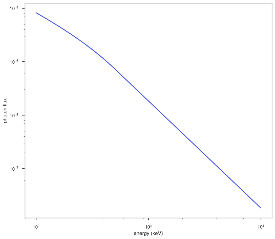
The shape of the function.

If this is not a photon model but a prior or linear function then ignore the units as these docs are auto-generated

fig, ax = plt.subplots()


ax.plot(energy_grid, func(energy_grid), color=blue)

ax.set_xlabel("energy (keV)")
ax.set_ylabel("photon flux")
ax.set_xscale(x_scale)
ax.set_yscale(y_scale)

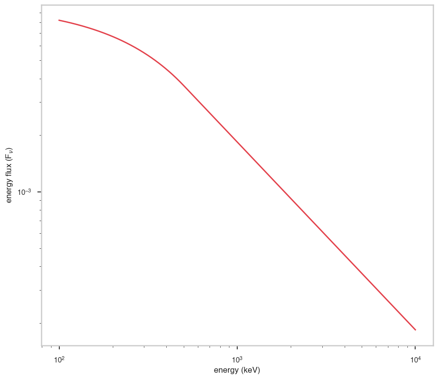
F\(_{\nu}\)

The F\(_{\nu}\) shape of the photon model if this is not a photon model, please ignore this auto-generated plot

fig, ax = plt.subplots()

ax.plot(energy_grid, energy_grid * func(energy_grid), red)


ax.set_xlabel("energy (keV)")
ax.set_ylabel(r"energy flux (F$_{\nu}$)")
ax.set_xscale(x_scale)
ax.set_yscale(y_scale)

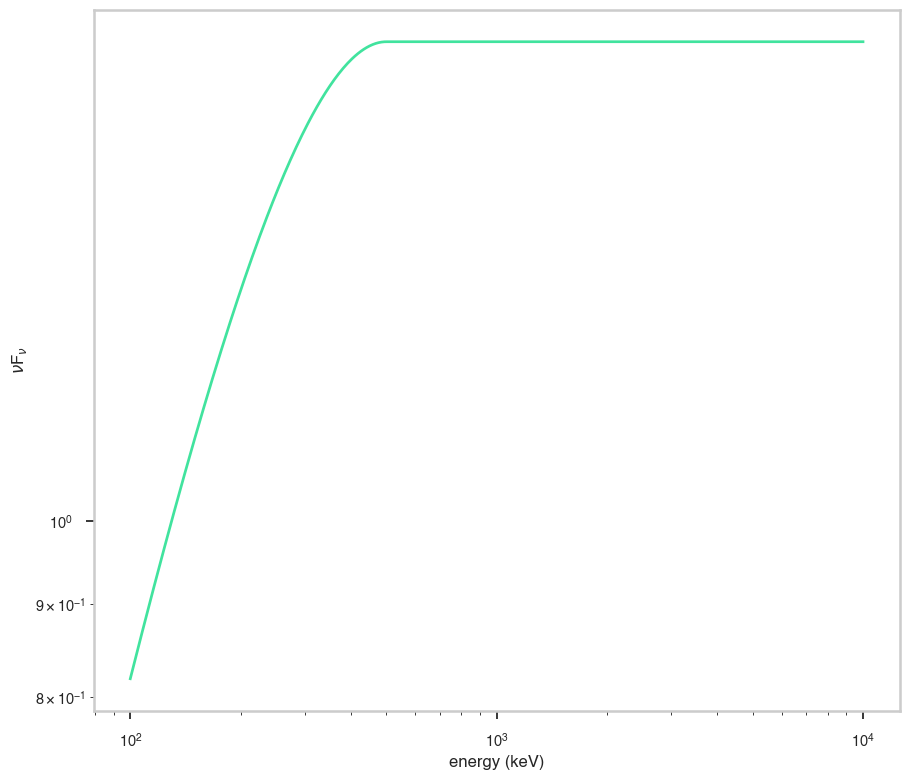
\(\nu\)F\(_{\nu}\)

The \(\nu\)F\(_{\nu}\) shape of the photon model if this is not a photon model, please ignore this auto-generated plot

fig, ax = plt.subplots()

ax.plot(energy_grid, energy_grid**2 * func(energy_grid), color=green)


ax.set_xlabel("energy (keV)")
ax.set_ylabel(r"$\nu$F$_{\nu}$")
ax.set_xscale(x_scale)
ax.set_yscale(y_scale)