Analyzing GRB 080916C with Fermi-GBM

Alt text (NASA/Swift/Cruz deWilde)

To demonstrate the capabilities and features of 3ML in, we will go through a time-integrated and time-resolved analysis. This example serves as a standard way to analyze Fermi-GBM data with 3ML as well as a template for how you can design your instrument’s analysis pipeline with 3ML if you have similar data.

3ML provides utilities to reduce time series data to plugins in a correct and statistically justified way (e.g., background fitting of Poisson data is done with a Poisson likelihood). The approach is generic and can be extended. For more details, see the time series documentation.

[1]:

import warnings

warnings.simplefilter("ignore")

[2]:

%%capture
import matplotlib.pyplot as plt
import numpy as np

np.seterr(all="ignore")


from threeML import *
from threeML.io.package_data import get_path_of_data_file

[3]:

silence_warnings()
%matplotlib inline
from jupyterthemes import jtplot

jtplot.style(context="talk", fscale=1, ticks=True, grid=False)
set_threeML_style()

Examining the catalog

As with Swift and Fermi-LAT, 3ML provides a simple interface to the on-line Fermi-GBM catalog. Let’s get the information for GRB 080916C.

[4]:

gbm_catalog = FermiGBMBurstCatalog()
gbm_catalog.query_sources("GRB080916009")

17:48:47 INFO      The cache for fermigbrst does not yet exist. We will try to    get_heasarc_table_as_pandas.py:63
                  build it

         INFO      Building cache for fermigbrst                                 get_heasarc_table_as_pandas.py:103

[4]:

Table length=1

name	ra	dec	trigger_time	t90
object	float64	float64	float64	float64
GRB080916009	119.800	-56.600	54725.0088613	62.977

To aid in quickly replicating the catalog analysis, and thanks to the tireless efforts of the Fermi-GBM team, we have added the ability to extract the analysis parameters from the catalog as well as build an astromodels model with the best fit parameters baked in. Using this information, one can quickly run through the catalog an replicate the entire analysis with a script. Let’s give it a try.

[5]:

grb_info = gbm_catalog.get_detector_information()["GRB080916009"]

gbm_detectors = grb_info["detectors"]
source_interval = grb_info["source"]["fluence"]
background_interval = grb_info["background"]["full"]
best_fit_model = grb_info["best fit model"]["fluence"]
model = gbm_catalog.get_model(best_fit_model, "fluence")["GRB080916009"]

[6]:

model

[6]:

Model summary:

	N
Point sources	1
Extended sources	0
Particle sources	0

Free parameters (5):

	value	min_value	max_value	unit
GRB080916009.spectrum.main.SmoothlyBrokenPowerLaw.K	0.012255	0.0	None	keV-1 s-1 cm-2
GRB080916009.spectrum.main.SmoothlyBrokenPowerLaw.alpha	-1.130424	-1.5	2.0
GRB080916009.spectrum.main.SmoothlyBrokenPowerLaw.break_energy	309.2031	10.0	None	keV
GRB080916009.spectrum.main.SmoothlyBrokenPowerLaw.break_scale	0.3	0.0	10.0
GRB080916009.spectrum.main.SmoothlyBrokenPowerLaw.beta	-2.096931	-5.0	-1.6

Fixed parameters (3):
(abridged. Use complete=True to see all fixed parameters)

Properties (0):

(none)

Linked parameters (0):

(none)

Independent variables:

(none)

Linked functions (0):

(none)

Downloading the data

We provide a simple interface to download the Fermi-GBM data. Using the information from the catalog that we have extracted, we can download just the data from the detectors that were used for the catalog analysis. This will download the CSPEC, TTE and instrument response files from the on-line database.

[7]:

dload = download_GBM_trigger_data("bn080916009", detectors=gbm_detectors)

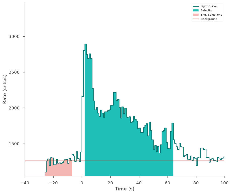
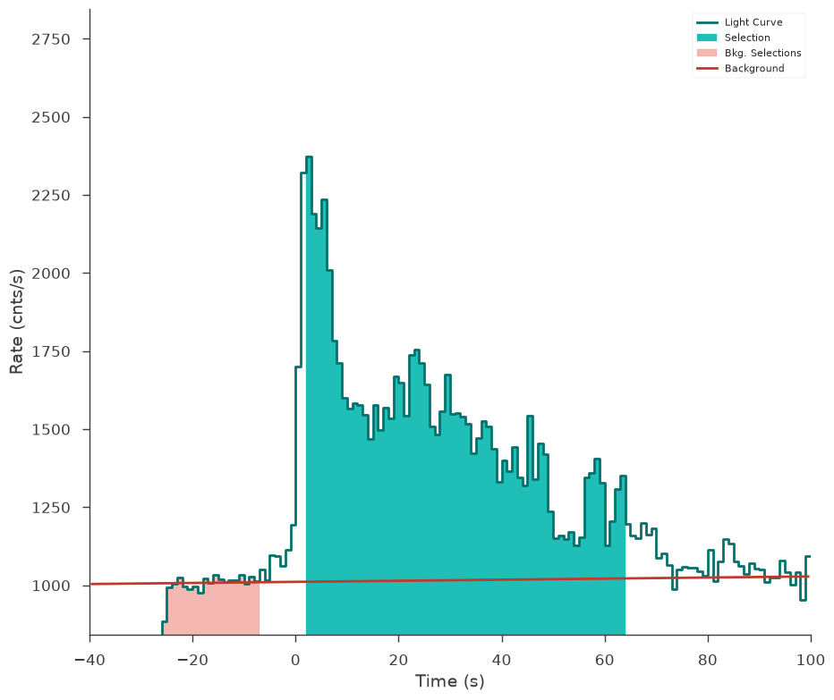
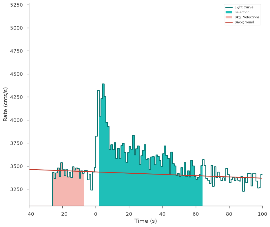
Let’s first examine the catalog fluence fit. Using the TimeSeriesBuilder, we can fit the background, set the source interval, and create a 3ML plugin for the analysis. We will loop through the detectors, set their appropriate channel selections, and ensure there are enough counts in each bin to make the PGStat profile likelihood valid.

First we use the CSPEC data to fit the background using the background selections. We use CSPEC because it has a longer duration for fitting the background.
The background is saved to an HDF5 file that stores the polynomial coefficients and selections which we can read in to the TTE file later.
The light curve is plotted.
The source selection from the catalog is set and DispersionSpectrumLike plugin is created.
The plugin has the standard GBM channel selections for spectral analysis set.

[8]:

fluence_plugins = []
time_series = {}
for det in gbm_detectors:

    ts_cspec = TimeSeriesBuilder.from_gbm_cspec_or_ctime(
        det, cspec_or_ctime_file=dload[det]["cspec"], rsp_file=dload[det]["rsp"]
    )

    ts_cspec.set_background_interval(*background_interval.split(","))
    ts_cspec.save_background(f"{det}_bkg.h5", overwrite=True)

    ts_tte = TimeSeriesBuilder.from_gbm_tte(
        det,
        tte_file=dload[det]["tte"],
        rsp_file=dload[det]["rsp"],
        restore_background=f"{det}_bkg.h5",
    )

    time_series[det] = ts_tte

    ts_tte.set_active_time_interval(source_interval)

    ts_tte.view_lightcurve(-40, 100)

    fluence_plugin = ts_tte.to_spectrumlike()

    if det.startswith("b"):

        fluence_plugin.set_active_measurements("250-30000")

    else:

        fluence_plugin.set_active_measurements("9-900")

    fluence_plugin.rebin_on_background(1.0)

    fluence_plugins.append(fluence_plugin)

17:49:30 INFO      Auto-determined polynomial order: 0                                binned_spectrum_series.py:356

17:49:35 INFO      None 0-order polynomial fit with the mle method                               time_series.py:426

         INFO      Saved fitted background to n3_bkg.h5                                          time_series.py:972

         INFO      Saved background to n3_bkg.h5                                         time_series_builder.py:430

17:49:36 INFO      Successfully restored fit from n3_bkg.h5                              time_series_builder.py:166

         INFO      Interval set to 1.28-64.257 for n3                                    time_series_builder.py:274

         INFO      Auto-probed noise models:                                                    SpectrumLike.py:486

         INFO      - observation: poisson                                                       SpectrumLike.py:487

         INFO      - background: gaussian                                                       SpectrumLike.py:488

         INFO      Range 9-900 translates to channels 5-124                                    SpectrumLike.py:1237

17:49:40 INFO      Now using 120 bins                                                          SpectrumLike.py:1706

17:49:41 INFO      Auto-determined polynomial order: 1                                binned_spectrum_series.py:356

17:49:47 INFO      None 1-order polynomial fit with the mle method                               time_series.py:426

         INFO      Saved fitted background to n4_bkg.h5                                          time_series.py:972

         INFO      Saved background to n4_bkg.h5                                         time_series_builder.py:430

17:49:48 INFO      Successfully restored fit from n4_bkg.h5                              time_series_builder.py:166

         INFO      Interval set to 1.28-64.257 for n4                                    time_series_builder.py:274

         INFO      Auto-probed noise models:                                                    SpectrumLike.py:486

         INFO      - observation: poisson                                                       SpectrumLike.py:487

         INFO      - background: gaussian                                                       SpectrumLike.py:488

         INFO      Range 9-900 translates to channels 5-123                                    SpectrumLike.py:1237

         INFO      Now using 119 bins                                                          SpectrumLike.py:1706

17:49:49 INFO      Auto-determined polynomial order: 1                                binned_spectrum_series.py:356

17:49:55 INFO      None 1-order polynomial fit with the mle method                               time_series.py:426

         INFO      Saved fitted background to b0_bkg.h5                                          time_series.py:972

         INFO      Saved background to b0_bkg.h5                                         time_series_builder.py:430

         INFO      Successfully restored fit from b0_bkg.h5                              time_series_builder.py:166

         INFO      Interval set to 1.28-64.257 for b0                                    time_series_builder.py:274

         INFO      Auto-probed noise models:                                                    SpectrumLike.py:486

         INFO      - observation: poisson                                                       SpectrumLike.py:487

         INFO      - background: gaussian                                                       SpectrumLike.py:488

         INFO      Range 250-30000 translates to channels 1-119                                SpectrumLike.py:1237

         INFO      Now using 119 bins                                                          SpectrumLike.py:1706

../_images/notebooks_grb080916C_12_42.png

../_images/notebooks_grb080916C_12_43.png

../_images/notebooks_grb080916C_12_44.png

Setting up the fit

Let’s see if we can reproduce the results from the catalog.

Set priors for the model

We will fit the spectrum using Bayesian analysis, so we must set priors on the model parameters.

[9]:

model.GRB080916009.spectrum.main.shape.alpha.prior = Truncated_gaussian(
    lower_bound=-1.5, upper_bound=1, mu=-1, sigma=0.5
)
model.GRB080916009.spectrum.main.shape.beta.prior = Truncated_gaussian(
    lower_bound=-5, upper_bound=-1.6, mu=-2.25, sigma=0.5
)
model.GRB080916009.spectrum.main.shape.break_energy.prior = Log_normal(mu=2, sigma=1)
model.GRB080916009.spectrum.main.shape.break_energy.bounds = (None, None)
model.GRB080916009.spectrum.main.shape.K.prior = Log_uniform_prior(
    lower_bound=1e-3, upper_bound=1e1
)
model.GRB080916009.spectrum.main.shape.break_scale.prior = Log_uniform_prior(
    lower_bound=1e-4, upper_bound=10
)

Clone the model and setup the Bayesian analysis class

Next, we clone the model we built from the catalog so that we can look at the results later and fit the cloned model. We pass this model and the DataList of the plugins to a BayesianAnalysis class and set the sampler to MultiNest.

[10]:

new_model = clone_model(model)

bayes = BayesianAnalysis(new_model, DataList(*fluence_plugins))

# share spectrum gives a linear speed up when
# spectrumlike plugins have the same RSP input energies
bayes.set_sampler("multinest", share_spectrum=True)

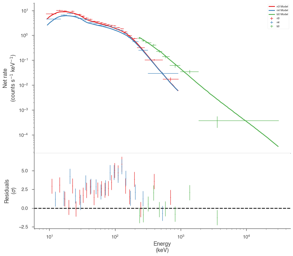
17:49:56 INFO      sampler set to multinest                                                bayesian_analysis.py:186

Examine at the catalog fitted model

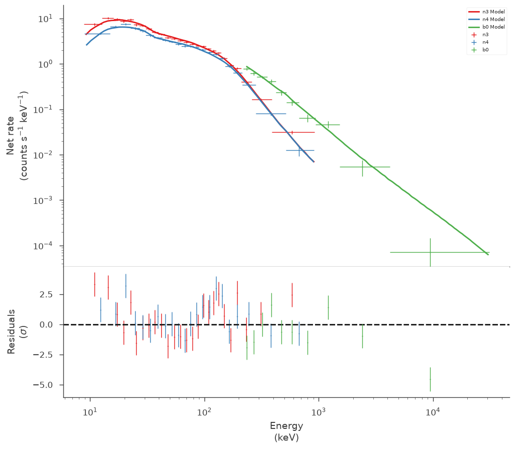
We can quickly examine how well the catalog fit matches the data. There appears to be a discrepancy between the data and the model! Let’s refit to see if we can fix it.

[11]:

fig = display_spectrum_model_counts(bayes, min_rate=20, step=False)

../_images/notebooks_grb080916C_18_0.png

Run the sampler

We let MultiNest condition the model on the data

[12]:

bayes.sampler.setup(n_live_points=400)
bayes.sample()

 *****************************************************
 MultiNest v3.10
 Copyright Farhan Feroz & Mike Hobson
 Release Jul 2015

 no. of live points =  400
 dimensionality =    5
 *****************************************************
  analysing data from chains/fit-.txt
 ln(ev)=  -3102.3287928265208      +/-  0.23204882326189835
 Total Likelihood Evaluations:        23112
 Sampling finished. Exiting MultiNest

17:50:08 INFO      fit restored to maximum of posterior                                         sampler_base.py:168

         INFO      fit restored to maximum of posterior                                         sampler_base.py:168

Maximum a posteriori probability (MAP) point:

	result	unit
parameter
GRB080916009...K	(1.447 +0.009 +0.05) x 10^-2	1 / (keV s cm2)
GRB080916009...alpha	-1.100 +0.009 +0.04
GRB080916009...break_energy	(1.91 +0.07 +0.5) x 10^2	keV
GRB080916009...break_scale	(0.0 +1.7 +3.0) x 10^-1
GRB080916009...beta	-1.94 -0.18 -0.06

Values of -log(posterior) at the minimum:

	-log(posterior)
n3	-1018.419563
n4	-1011.828426
b0	-1051.522757
total	-3081.770746

Values of statistical measures:

	statistical measures
AIC	6173.711947
BIC	6192.944158
DIC	6178.808911
PDIC	4.000334
log(Z)	-1347.324276

Now our model seems to match much better with the data!

[13]:

bayes.restore_median_fit()
fig = display_spectrum_model_counts(bayes, min_rate=20)

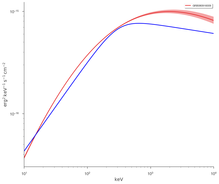
         INFO      fit restored to median of posterior                                          sampler_base.py:157

../_images/notebooks_grb080916C_22_1.png

But how different are we from the catalog model? Let’s plot our fit along with the catalog model. Luckily, 3ML can handle all the units for is

[14]:

conversion = u.Unit("keV2/(cm2 s keV)").to("erg2/(cm2 s keV)")
energy_grid = np.logspace(1, 4, 100) * u.keV
vFv = (energy_grid**2 * model.get_point_source_fluxes(0, energy_grid)).to(
    "erg2/(cm2 s keV)"
)

[15]:

fig = plot_spectra(bayes.results, flux_unit="erg2/(cm2 s keV)")
ax = fig.get_axes()[0]
_ = ax.loglog(energy_grid, vFv, color="blue", label="catalog model")

../_images/notebooks_grb080916C_25_2.png

Time Resolved Analysis

Now that we have examined fluence fit, we can move to performing a time-resolved analysis.

Selecting a temporal binning

We first get the brightest NaI detector and create time bins via the Bayesian blocks algorithm. We can use the fitted background to make sure that our intervals are chosen in an unbiased way.

[16]:

n3 = time_series["n3"]

[17]:

n3.create_time_bins(0, 60, method="bayesblocks", use_background=True, p0=0.2)

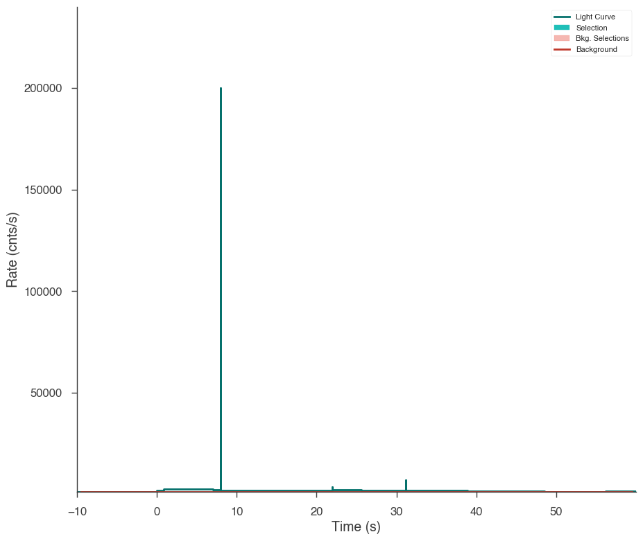
17:51:05 INFO      Created 15 bins via bayesblocks                                       time_series_builder.py:632

Sometimes, glitches in the GBM data cause spikes in the data that the Bayesian blocks algorithm detects as fast changes in the count rate. We will have to remove those intervals manually.

Note: In the future, 3ML will provide an automated method to remove these unwanted spikes.

[18]:

fig = n3.view_lightcurve(use_binner=True)

../_images/notebooks_grb080916C_30_0.png

[19]:

bad_bins = []
for i, w in enumerate(n3.bins.widths):

    if w < 5e-2:
        bad_bins.append(i)

edges = [n3.bins.starts[0]]

for i, b in enumerate(n3.bins):

    if i not in bad_bins:
        edges.append(b.stop)

starts = edges[:-1]
stops = edges[1:]

n3.create_time_bins(starts, stops, method="custom")

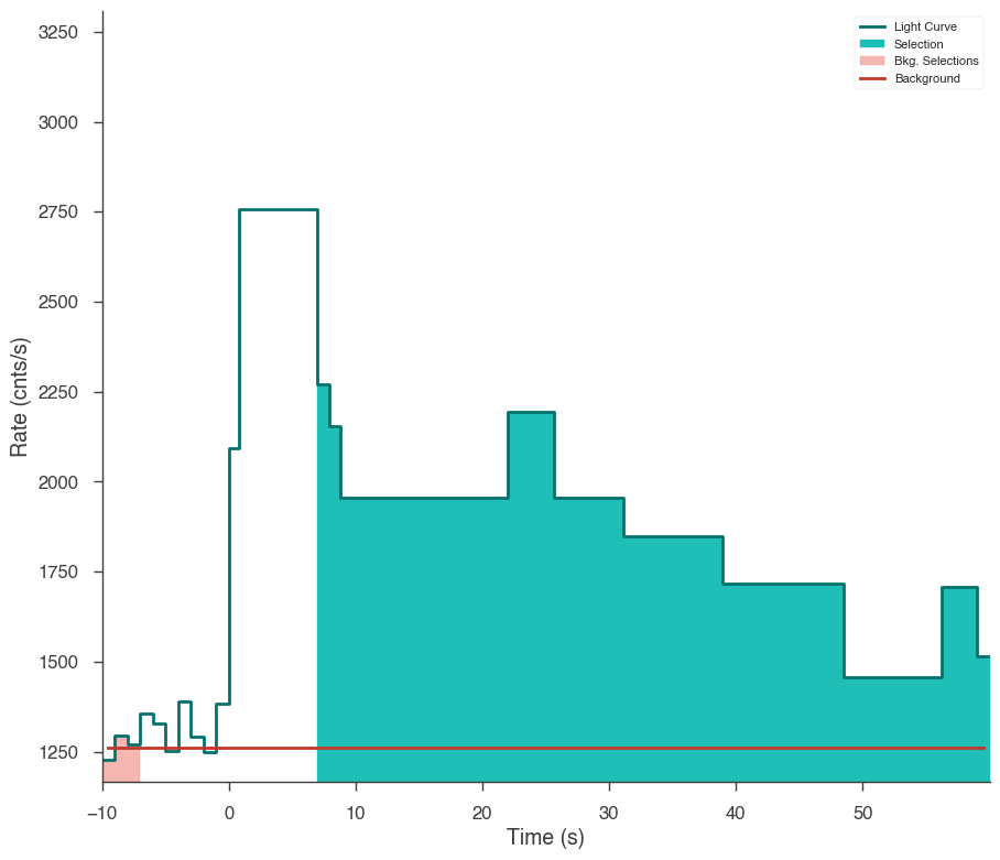
         INFO      Created 12 bins via custom                                            time_series_builder.py:632

Now our light curve looks much more acceptable.

[20]:

fig = n3.view_lightcurve(use_binner=True)

../_images/notebooks_grb080916C_33_0.png

The time series objects can read time bins from each other, so we will map these time bins onto the other detectors’ time series and create a list of time plugins for each detector and each time bin created above.

[21]:

time_resolved_plugins = {}

for k, v in time_series.items():
    v.read_bins(n3)
    time_resolved_plugins[k] = v.to_spectrumlike(from_bins=True)

         INFO      Created 12 bins via custom                                            time_series_builder.py:632

         INFO      Interval set to 1.28-64.257 for n3                                    time_series_builder.py:274

         INFO      Created 12 bins via custom                                            time_series_builder.py:632

17:51:06 INFO      Interval set to 1.28-64.257 for n4                                    time_series_builder.py:274

         INFO      Created 12 bins via custom                                            time_series_builder.py:632

         INFO      Interval set to 1.28-64.257 for b0                                    time_series_builder.py:274

Setting up the model

For the time-resolved analysis, we will fit the classic Band function to the data. We will set some principled priors.

[22]:

band = Band()
band.alpha.prior = Truncated_gaussian(lower_bound=-1.5, upper_bound=1, mu=-1, sigma=0.5)
band.beta.prior = Truncated_gaussian(lower_bound=-5, upper_bound=-1.6, mu=-2, sigma=0.5)
band.xp.prior = Log_normal(mu=2, sigma=1)
band.xp.bounds = (None, None)
band.K.prior = Log_uniform_prior(lower_bound=1e-10, upper_bound=1e3)
ps = PointSource("grb", 0, 0, spectral_shape=band)
band_model = Model(ps)

Perform the fits

One way to perform Bayesian spectral fits to all the intervals is to loop through each one. There can are many ways to do this, so find an analysis pattern that works for you.

[23]:

models = []
results = []
analysis = []
for interval in range(12):

    # clone the model above so that we have a separate model
    # for each fit

    this_model = clone_model(band_model)

    # for each detector set up the plugin
    # for this time interval

    this_data_list = []
    for k, v in time_resolved_plugins.items():

        pi = v[interval]

        if k.startswith("b"):
            pi.set_active_measurements("250-30000")
        else:
            pi.set_active_measurements("9-900")

        pi.rebin_on_background(1.0)

        this_data_list.append(pi)

    # create a data list

    dlist = DataList(*this_data_list)

    # set up the sampler and fit

    bayes = BayesianAnalysis(this_model, dlist)

    # get some speed with share spectrum
    bayes.set_sampler("multinest", share_spectrum=True)
    bayes.sampler.setup(n_live_points=500)
    bayes.sample()

    # at this stage we coudl also
    # save the analysis result to
    # disk but we will simply hold
    # onto them in memory

    analysis.append(bayes)

         INFO      Range 9-900 translates to channels 5-124                                    SpectrumLike.py:1237

         INFO      Now using 120 bins                                                          SpectrumLike.py:1706

         INFO      Range 9-900 translates to channels 5-123                                    SpectrumLike.py:1237

         INFO      Now using 119 bins                                                          SpectrumLike.py:1706

         INFO      Range 250-30000 translates to channels 1-119                                SpectrumLike.py:1237

         INFO      Now using 107 bins                                                          SpectrumLike.py:1706

         INFO      sampler set to multinest                                                bayesian_analysis.py:186

 *****************************************************
 MultiNest v3.10
 Copyright Farhan Feroz & Mike Hobson
 Release Jul 2015

 no. of live points =  500
 dimensionality =    4
 *****************************************************
  analysing data from chains/fit-.txt
 ln(ev)=  -788.98115828716936      +/-  0.18001349841787101
 Total Likelihood Evaluations:        15782
 Sampling finished. Exiting MultiNest

17:51:16 INFO      fit restored to maximum of posterior                                         sampler_base.py:168

         INFO      fit restored to maximum of posterior                                         sampler_base.py:168

Maximum a posteriori probability (MAP) point:

	result	unit
parameter
grb.spectrum.main.Band.K	(3.6 -0.5 +0.7) x 10^-2	1 / (keV s cm2)
grb.spectrum.main.Band.alpha	(-5.5 -1.3 +1.2) x 10^-1
grb.spectrum.main.Band.xp	(3.2 -0.5 +0.7) x 10^2	keV
grb.spectrum.main.Band.beta	-2.07 -0.20 +0.13

Values of -log(posterior) at the minimum:

	-log(posterior)
n3_interval0	-250.200647
n4_interval0	-268.062049
b0_interval0	-285.677384
total	-803.940080

Values of statistical measures:

	statistical measures
AIC	1615.993474
BIC	1631.402291
DIC	1569.746474
PDIC	2.119401
log(Z)	-342.650163

         INFO      Range 9-900 translates to channels 5-124                                    SpectrumLike.py:1237

         INFO      Now using 120 bins                                                          SpectrumLike.py:1706

         INFO      Range 9-900 translates to channels 5-123                                    SpectrumLike.py:1237

         INFO      Now using 119 bins                                                          SpectrumLike.py:1706

         INFO      Range 250-30000 translates to channels 1-119                                SpectrumLike.py:1237

         INFO      Now using 119 bins                                                          SpectrumLike.py:1706

         INFO      sampler set to multinest                                                bayesian_analysis.py:186

 *****************************************************
 MultiNest v3.10
 Copyright Farhan Feroz & Mike Hobson
 Release Jul 2015

 no. of live points =  500
 dimensionality =    4
 *****************************************************
  analysing data from chains/fit-.txt ln(ev)=  -1944.0973516181591      +/-  0.21636301376492745
 Total Likelihood Evaluations:        26049
 Sampling finished. Exiting MultiNest

17:51:30 INFO      fit restored to maximum of posterior                                         sampler_base.py:168

         INFO      fit restored to maximum of posterior                                         sampler_base.py:168

Maximum a posteriori probability (MAP) point:

	result	unit
parameter
grb.spectrum.main.Band.K	(4.11 -0.04 +0.21) x 10^-2	1 / (keV s cm2)
grb.spectrum.main.Band.alpha	(-8.59 -0.08 +0.4) x 10^-1
grb.spectrum.main.Band.xp	(6.26 -0.7 +0.12) x 10^2	keV
grb.spectrum.main.Band.beta	-2.147 -0.005 +0.10

Values of -log(posterior) at the minimum:

	-log(posterior)
n3_interval1	-641.888952
n4_interval1	-645.527626
b0_interval1	-673.824045
total	-1961.240623

Values of statistical measures:

	statistical measures
AIC	3930.594560
BIC	3946.003378
DIC	3871.992920
PDIC	2.886839
log(Z)	-844.310752

         INFO      Range 9-900 translates to channels 5-124                                    SpectrumLike.py:1237

         INFO      Now using 120 bins                                                          SpectrumLike.py:1706

         INFO      Range 9-900 translates to channels 5-123                                    SpectrumLike.py:1237

         INFO      Now using 119 bins                                                          SpectrumLike.py:1706

         INFO      Range 250-30000 translates to channels 1-119                                SpectrumLike.py:1237

         INFO      Now using 115 bins                                                          SpectrumLike.py:1706

         INFO      sampler set to multinest                                                bayesian_analysis.py:186

 *****************************************************
 MultiNest v3.10
 Copyright Farhan Feroz & Mike Hobson
 Release Jul 2015

 no. of live points =  500
 dimensionality =    4
 *****************************************************
 ln(ev)=  -918.37307721633044      +/-  0.18775706713785112
  analysing data from chains/fit-.txt
 Total Likelihood Evaluations:        18672
 Sampling finished. Exiting MultiNest

17:51:42 INFO      fit restored to maximum of posterior                                         sampler_base.py:168

         INFO      fit restored to maximum of posterior                                         sampler_base.py:168

Maximum a posteriori probability (MAP) point:

	result	unit
parameter
grb.spectrum.main.Band.K	(5.2 +0.4 +2.3) x 10^-2	1 / (keV s cm2)
grb.spectrum.main.Band.alpha	(-6.67 +0.06 +1.9) x 10^-1
grb.spectrum.main.Band.xp	(1.61 -0.4 -0.11) x 10^2	keV
grb.spectrum.main.Band.beta	-1.6067 -0.011 +0.0025

Values of -log(posterior) at the minimum:

	-log(posterior)
n3_interval2	-290.082283
n4_interval2	-309.775826
b0_interval2	-322.851130
total	-922.709239

Values of statistical measures:

	statistical measures
AIC	1853.531792
BIC	1868.940610
DIC	1818.481084
PDIC	1.014108
log(Z)	-398.844360

         INFO      Range 9-900 translates to channels 5-124                                    SpectrumLike.py:1237

         INFO      Now using 120 bins                                                          SpectrumLike.py:1706

         INFO      Range 9-900 translates to channels 5-123                                    SpectrumLike.py:1237

         INFO      Now using 119 bins                                                          SpectrumLike.py:1706

         INFO      Range 250-30000 translates to channels 1-119                                SpectrumLike.py:1237

         INFO      Now using 109 bins                                                          SpectrumLike.py:1706

         INFO      sampler set to multinest                                                bayesian_analysis.py:186

 *****************************************************
 MultiNest v3.10
 Copyright Farhan Feroz & Mike Hobson
 Release Jul 2015

 no. of live points =  500
 dimensionality =    4
 *****************************************************
  analysing data from chains/fit-.txt ln(ev)=  -791.74849609142427      +/-  0.18606579710910928
 Total Likelihood Evaluations:        17185
 Sampling finished. Exiting MultiNest

17:51:52 INFO      fit restored to maximum of posterior                                         sampler_base.py:168

         INFO      fit restored to maximum of posterior                                         sampler_base.py:168

Maximum a posteriori probability (MAP) point:

	result	unit
parameter
grb.spectrum.main.Band.K	(3.04 -0.22 +0.6) x 10^-2	1 / (keV s cm2)
grb.spectrum.main.Band.alpha	(-9.0 -0.6 +1.0) x 10^-1
grb.spectrum.main.Band.xp	(3.04 -0.7 +0.21) x 10^2	keV
grb.spectrum.main.Band.beta	-1.953 -0.006 +0.13

Values of -log(posterior) at the minimum:

	-log(posterior)
n3_interval3	-242.022201
n4_interval3	-262.213243
b0_interval3	-298.620579
total	-802.856023

Values of statistical measures:

	statistical measures
AIC	1613.825360
BIC	1629.234177
DIC	1570.554831
PDIC	2.081916
log(Z)	-343.852003

17:51:53 INFO      Range 9-900 translates to channels 5-124                                    SpectrumLike.py:1237

         INFO      Now using 120 bins                                                          SpectrumLike.py:1706

         INFO      Range 9-900 translates to channels 5-123                                    SpectrumLike.py:1237

         INFO      Now using 119 bins                                                          SpectrumLike.py:1706

         INFO      Range 250-30000 translates to channels 1-119                                SpectrumLike.py:1237

         INFO      Now using 119 bins                                                          SpectrumLike.py:1706

         INFO      sampler set to multinest                                                bayesian_analysis.py:186

 *****************************************************
 MultiNest v3.10
 Copyright Farhan Feroz & Mike Hobson
 Release Jul 2015

 no. of live points =  500
 dimensionality =    4
 *****************************************************
  analysing data from chains/fit-.txt
 ln(ev)=  -2298.2436335744364      +/-  0.21553401248919346
 Total Likelihood Evaluations:        21429
 Sampling finished. Exiting MultiNest

17:52:06 INFO      fit restored to maximum of posterior                                         sampler_base.py:168

         INFO      fit restored to maximum of posterior                                         sampler_base.py:168

Maximum a posteriori probability (MAP) point:

	result	unit
parameter
grb.spectrum.main.Band.K	(2.089 -0.20 +0.014) x 10^-2	1 / (keV s cm2)
grb.spectrum.main.Band.alpha	-1.046 -0.07 +0.007
grb.spectrum.main.Band.xp	(3.90 -0.10 +0.9) x 10^2	keV
grb.spectrum.main.Band.beta	-2.69 -0.10 +0.15

Values of -log(posterior) at the minimum:

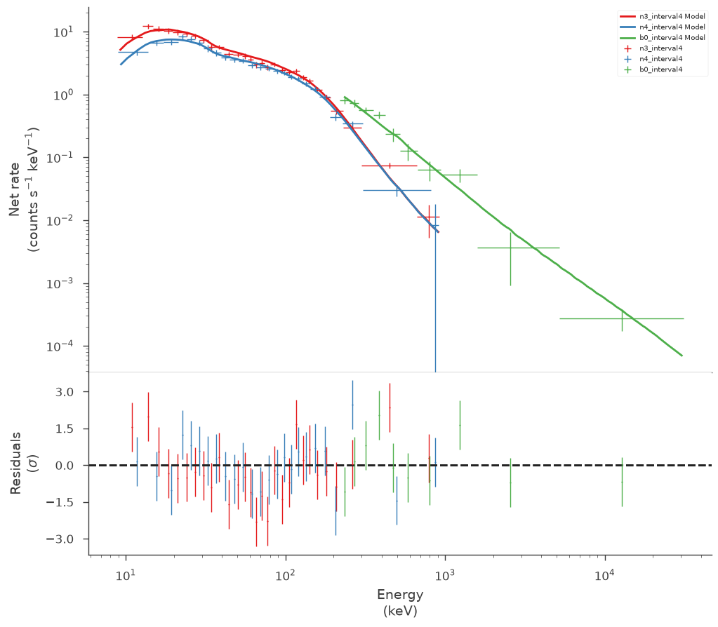
	-log(posterior)
n3_interval4	-769.265701
n4_interval4	-752.617150
b0_interval4	-787.251792
total	-2309.134644

Values of statistical measures:

	statistical measures
AIC	4626.382602
BIC	4641.791420
DIC	4577.114397
PDIC	2.438043
log(Z)	-998.114528

         INFO      Range 9-900 translates to channels 5-124                                    SpectrumLike.py:1237

         INFO      Now using 120 bins                                                          SpectrumLike.py:1706

         INFO      Range 9-900 translates to channels 5-123                                    SpectrumLike.py:1237

         INFO      Now using 119 bins                                                          SpectrumLike.py:1706

         INFO      Range 250-30000 translates to channels 1-119                                SpectrumLike.py:1237

         INFO      Now using 119 bins                                                          SpectrumLike.py:1706

         INFO      sampler set to multinest                                                bayesian_analysis.py:186

 *****************************************************
 MultiNest v3.10
 Copyright Farhan Feroz & Mike Hobson
 Release Jul 2015

 no. of live points =  500
 dimensionality =    4
 *****************************************************
  analysing data from chains/fit-.txt ln(ev)=  -1575.1165003685330      +/-  0.19630627877253565
 Total Likelihood Evaluations:        21620
 Sampling finished. Exiting MultiNest

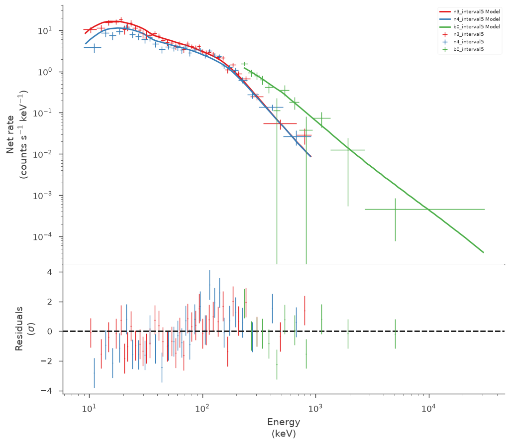
17:52:18 INFO      fit restored to maximum of posterior                                         sampler_base.py:168

         INFO      fit restored to maximum of posterior                                         sampler_base.py:168

Maximum a posteriori probability (MAP) point:

	result	unit
parameter
grb.spectrum.main.Band.K	(2.88 +0.07 +0.32) x 10^-2	1 / (keV s cm2)
grb.spectrum.main.Band.alpha	(-8.90 +0.19 +0.8) x 10^-1
grb.spectrum.main.Band.xp	(3.96 -0.6 -0.05) x 10^2	keV
grb.spectrum.main.Band.beta	-2.08 -0.15 +0.07

Values of -log(posterior) at the minimum:

	-log(posterior)
n3_interval5	-523.758676
n4_interval5	-527.357612
b0_interval5	-536.396053
total	-1587.512341

Values of statistical measures:

	statistical measures
AIC	3183.137996
BIC	3198.546814
DIC	3136.384502
PDIC	2.580008
log(Z)	-684.064404

         INFO      Range 9-900 translates to channels 5-124                                    SpectrumLike.py:1237

         INFO      Now using 120 bins                                                          SpectrumLike.py:1706

         INFO      Range 9-900 translates to channels 5-123                                    SpectrumLike.py:1237

         INFO      Now using 119 bins                                                          SpectrumLike.py:1706

         INFO      Range 250-30000 translates to channels 1-119                                SpectrumLike.py:1237

         INFO      Now using 119 bins                                                          SpectrumLike.py:1706

         INFO      sampler set to multinest                                                bayesian_analysis.py:186

 *****************************************************
 MultiNest v3.10
 Copyright Farhan Feroz & Mike Hobson
 Release Jul 2015

 no. of live points =  500
 dimensionality =    4
 *****************************************************
  analysing data from chains/fit-.txt ln(ev)=  -1756.1615191398546      +/-  0.19754167281929805
 Total Likelihood Evaluations:        20480
 Sampling finished. Exiting MultiNest

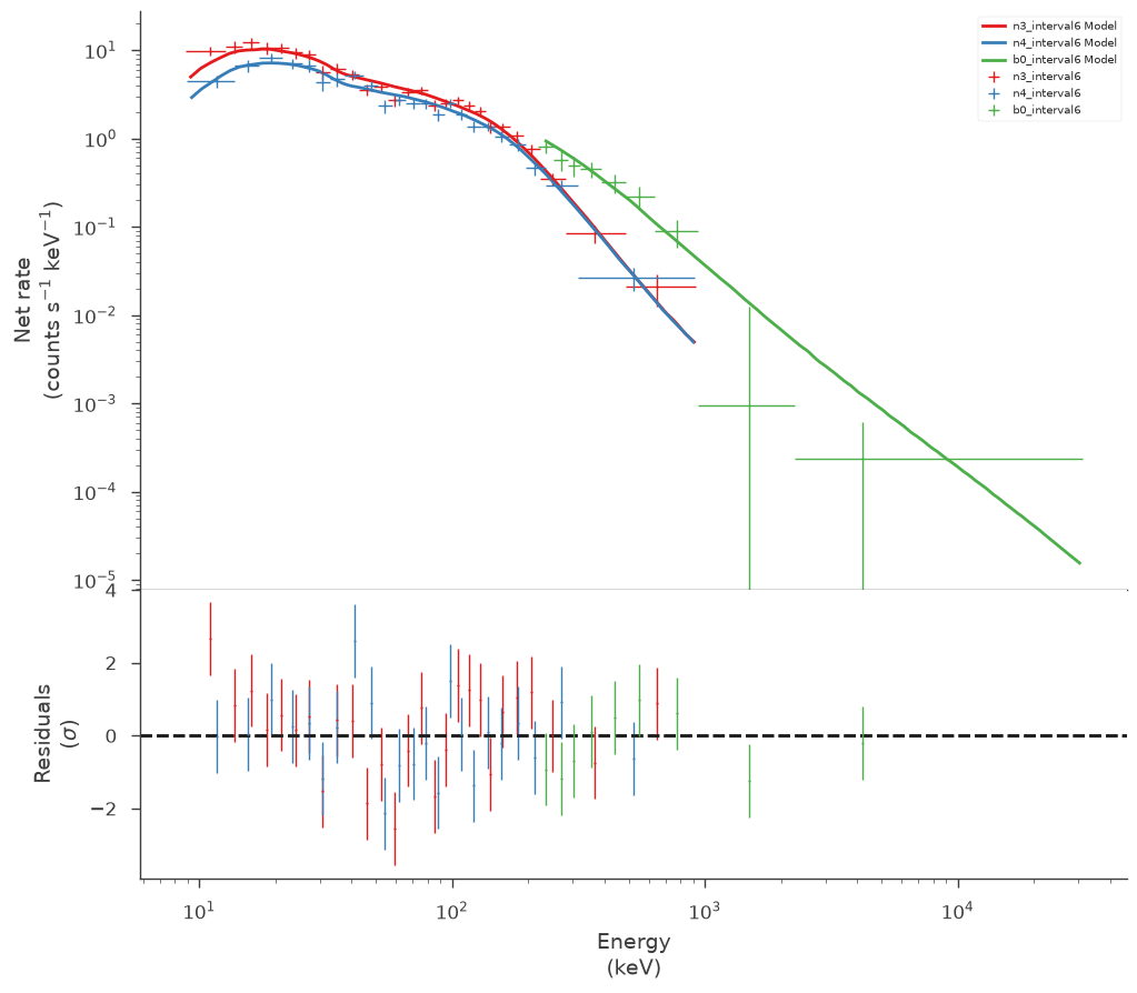
17:52:30 INFO      fit restored to maximum of posterior                                         sampler_base.py:168

         INFO      fit restored to maximum of posterior                                         sampler_base.py:168

Maximum a posteriori probability (MAP) point:

	result	unit
parameter
grb.spectrum.main.Band.K	(1.927 -0.033 +0.19) x 10^-2	1 / (keV s cm2)
grb.spectrum.main.Band.alpha	-1.015 -0.012 +0.06
grb.spectrum.main.Band.xp	(4.63 -0.8 +0.25) x 10^2	keV
grb.spectrum.main.Band.beta	-2.387 -0.5 -0.015

Values of -log(posterior) at the minimum:

	-log(posterior)
n3_interval6	-584.342825
n4_interval6	-577.058891
b0_interval6	-609.769241
total	-1771.170956

Values of statistical measures:

	statistical measures
AIC	3550.455227
BIC	3565.864045
DIC	3500.506427
PDIC	2.533898
log(Z)	-762.691257

         INFO      Range 9-900 translates to channels 5-124                                    SpectrumLike.py:1237

         INFO      Now using 120 bins                                                          SpectrumLike.py:1706

         INFO      Range 9-900 translates to channels 5-123                                    SpectrumLike.py:1237

         INFO      Now using 119 bins                                                          SpectrumLike.py:1706

         INFO      Range 250-30000 translates to channels 1-119                                SpectrumLike.py:1237

         INFO      Now using 119 bins                                                          SpectrumLike.py:1706

         INFO      sampler set to multinest                                                bayesian_analysis.py:186

 *****************************************************
 MultiNest v3.10
 Copyright Farhan Feroz & Mike Hobson
 Release Jul 2015

 no. of live points =  500
 dimensionality =    4
 *****************************************************
  analysing data from chains/fit-.txt ln(ev)=  -1944.1329165264601      +/-  0.19996508003421154
 Total Likelihood Evaluations:        19517
 Sampling finished. Exiting MultiNest

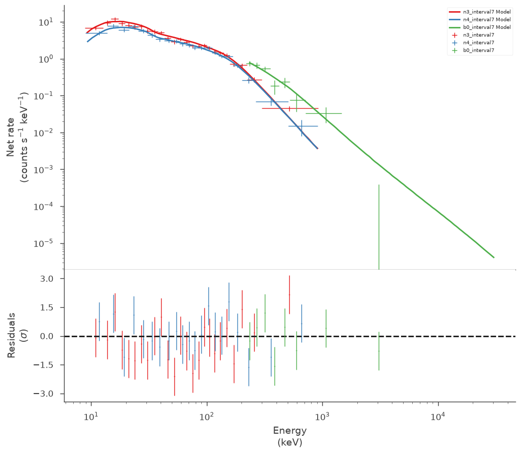
17:52:41 INFO      fit restored to maximum of posterior                                         sampler_base.py:168

         INFO      fit restored to maximum of posterior                                         sampler_base.py:168

Maximum a posteriori probability (MAP) point:

	result	unit
parameter
grb.spectrum.main.Band.K	(1.5700 -0.0013 +0.4) x 10^-2	1 / (keV s cm2)
grb.spectrum.main.Band.alpha	-1.110 -0.021 +0.18
grb.spectrum.main.Band.xp	(4.88 -1.9 +0.04) x 10^2	keV
grb.spectrum.main.Band.beta	-2.23 -0.4 +0.27

Values of -log(posterior) at the minimum:

	-log(posterior)
n3_interval7	-641.919900
n4_interval7	-650.944692
b0_interval7	-663.177415
total	-1956.042007

Values of statistical measures:

	statistical measures
AIC	3920.197328
BIC	3935.606145
DIC	3875.397155
PDIC	4.426218
log(Z)	-844.326198

         INFO      Range 9-900 translates to channels 5-124                                    SpectrumLike.py:1237

         INFO      Now using 120 bins                                                          SpectrumLike.py:1706

         INFO      Range 9-900 translates to channels 5-123                                    SpectrumLike.py:1237

         INFO      Now using 119 bins                                                          SpectrumLike.py:1706

         INFO      Range 250-30000 translates to channels 1-119                                SpectrumLike.py:1237

         INFO      Now using 119 bins                                                          SpectrumLike.py:1706

         INFO      sampler set to multinest                                                bayesian_analysis.py:186

 *****************************************************
 MultiNest v3.10
 Copyright Farhan Feroz & Mike Hobson
 Release Jul 2015

 no. of live points =  500
 dimensionality =    4
 *****************************************************
  analysing data from chains/fit-.txt ln(ev)=  -2054.2106090713560      +/-  0.19081821145859992
 Total Likelihood Evaluations:        18875
 Sampling finished. Exiting MultiNest

17:52:52 INFO      fit restored to maximum of posterior                                         sampler_base.py:168

         INFO      fit restored to maximum of posterior                                         sampler_base.py:168

Maximum a posteriori probability (MAP) point:

	result	unit
parameter
grb.spectrum.main.Band.K	(1.53 -0.12 +0.09) x 10^-2	1 / (keV s cm2)
grb.spectrum.main.Band.alpha	(-8.5 -0.6 +0.5) x 10^-1
grb.spectrum.main.Band.xp	(3.73 -0.28 +0.7) x 10^2	keV
grb.spectrum.main.Band.beta	-2.32 -0.4 +0.06

Values of -log(posterior) at the minimum:

	-log(posterior)
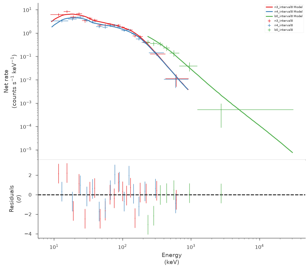
n3_interval8	-698.420623
n4_interval8	-666.333788
b0_interval8	-702.074909
total	-2066.829320

Values of statistical measures:

	statistical measures
AIC	4141.771954
BIC	4157.180772
DIC	4097.174589
PDIC	2.764043
log(Z)	-892.132332

         INFO      Range 9-900 translates to channels 5-124                                    SpectrumLike.py:1237

         INFO      Now using 120 bins                                                          SpectrumLike.py:1706

         INFO      Range 9-900 translates to channels 5-123                                    SpectrumLike.py:1237

         INFO      Now using 119 bins                                                          SpectrumLike.py:1706

         INFO      Range 250-30000 translates to channels 1-119                                SpectrumLike.py:1237

         INFO      Now using 119 bins                                                          SpectrumLike.py:1706

         INFO      sampler set to multinest                                                bayesian_analysis.py:186

 *****************************************************
 MultiNest v3.10
 Copyright Farhan Feroz & Mike Hobson
 Release Jul 2015

 no. of live points =  500
 dimensionality =    4
 *****************************************************
  analysing data from chains/fit-.txt ln(ev)=  -1878.1963560044071      +/-  0.14185630903023605
 Total Likelihood Evaluations:        14353
 Sampling finished. Exiting MultiNest

17:52:58 INFO      fit restored to maximum of posterior                                         sampler_base.py:168

         INFO      fit restored to maximum of posterior                                         sampler_base.py:168

Maximum a posteriori probability (MAP) point:

	result	unit
parameter
grb.spectrum.main.Band.K	(1.1 -0.4 +1.0) x 10^-2	1 / (keV s cm2)
grb.spectrum.main.Band.alpha	(-8.5 -2.1 +2.9) x 10^-1
grb.spectrum.main.Band.xp	(1.2 -0.4 +0.6) x 10^2	keV
grb.spectrum.main.Band.beta	-1.85 -0.4 +0.11

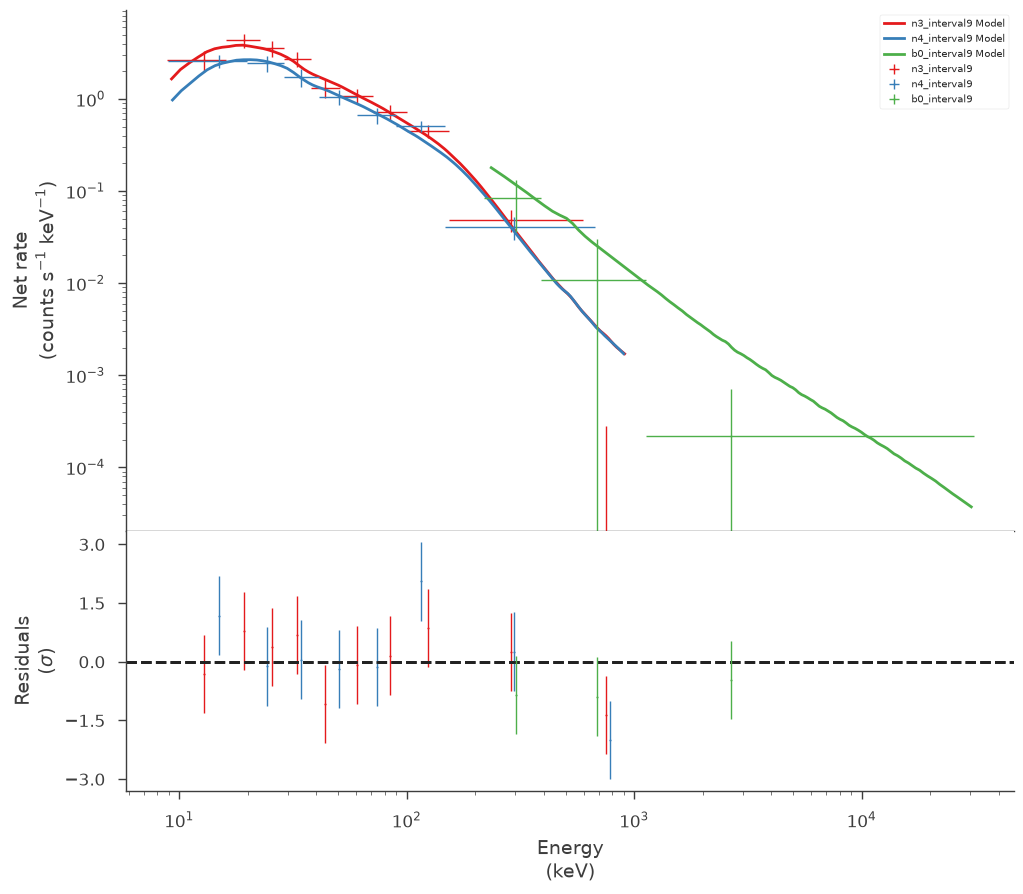
Values of -log(posterior) at the minimum:

	-log(posterior)
n3_interval9	-616.981579
n4_interval9	-616.257369
b0_interval9	-648.574460
total	-1881.813409

Values of statistical measures:

	statistical measures
AIC	3771.740132
BIC	3787.148949
DIC	3706.823874
PDIC	-40.424500
log(Z)	-815.690313

         INFO      Range 9-900 translates to channels 5-124                                    SpectrumLike.py:1237

         INFO      Now using 120 bins                                                          SpectrumLike.py:1706

         INFO      Range 9-900 translates to channels 5-123                                    SpectrumLike.py:1237

         INFO      Now using 119 bins                                                          SpectrumLike.py:1706

         INFO      Range 250-30000 translates to channels 1-119                                SpectrumLike.py:1237

         INFO      Now using 119 bins                                                          SpectrumLike.py:1706

         INFO      sampler set to multinest                                                bayesian_analysis.py:186

 *****************************************************
 MultiNest v3.10
 Copyright Farhan Feroz & Mike Hobson
 Release Jul 2015

 no. of live points =  500
 dimensionality =    4
 *****************************************************
  analysing data from chains/fit-.txt ln(ev)=  -1323.2247160158227      +/-  0.17224000498296418
 Total Likelihood Evaluations:        15414
 Sampling finished. Exiting MultiNest

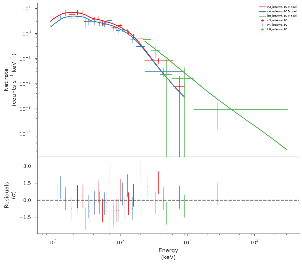
17:53:08 INFO      fit restored to maximum of posterior                                         sampler_base.py:168

         INFO      fit restored to maximum of posterior                                         sampler_base.py:168

Maximum a posteriori probability (MAP) point:

	result	unit
parameter
grb.spectrum.main.Band.K	(2.2 +/- 0.5) x 10^-2	1 / (keV s cm2)
grb.spectrum.main.Band.alpha	(-7.0 -1.8 +0.9) x 10^-1
grb.spectrum.main.Band.xp	(2.02 -0.34 +0.7) x 10^2	keV
grb.spectrum.main.Band.beta	-1.89 -0.32 +0.11

Values of -log(posterior) at the minimum:

	-log(posterior)
n3_interval10	-437.608925
n4_interval10	-432.904470
b0_interval10	-460.832595
total	-1331.345990

Values of statistical measures:

	statistical measures
AIC	2670.805295
BIC	2686.214113
DIC	2633.961378
PDIC	0.450744
log(Z)	-574.669192

         INFO      Range 9-900 translates to channels 5-124                                    SpectrumLike.py:1237

         INFO      Now using 120 bins                                                          SpectrumLike.py:1706

         INFO      Range 9-900 translates to channels 5-123                                    SpectrumLike.py:1237

         INFO      Now using 119 bins                                                          SpectrumLike.py:1706

         INFO      Range 250-30000 translates to channels 1-119                                SpectrumLike.py:1237

         INFO      Now using 119 bins                                                          SpectrumLike.py:1706

         INFO      sampler set to multinest                                                bayesian_analysis.py:186

 *****************************************************
 MultiNest v3.10
 Copyright Farhan Feroz & Mike Hobson
 Release Jul 2015

 no. of live points =  500
 dimensionality =    4
 *****************************************************
  analysing data from chains/fit-.txt ln(ev)=  -812.11105456371774      +/-  0.14896314800182525
 Total Likelihood Evaluations:        11733
 Sampling finished. Exiting MultiNest

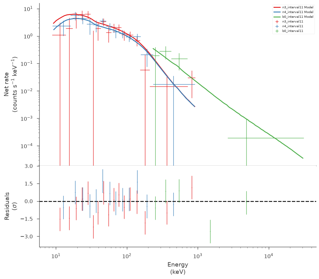
17:53:15 INFO      fit restored to maximum of posterior                                         sampler_base.py:168

         INFO      fit restored to maximum of posterior                                         sampler_base.py:168

Maximum a posteriori probability (MAP) point:

	result	unit
parameter
grb.spectrum.main.Band.K	(2.7 -0.7 +1.9) x 10^-2	1 / (keV s cm2)
grb.spectrum.main.Band.alpha	(-4.9 -1.9 +3.1) x 10^-1
grb.spectrum.main.Band.xp	(1.32 -0.31 +0.29) x 10^2	keV
grb.spectrum.main.Band.beta	-2.15 -0.5 +0.17

Values of -log(posterior) at the minimum:

	-log(posterior)
n3_interval11	-272.353537
n4_interval11	-255.936948
b0_interval11	-292.420995
total	-820.711479

Values of statistical measures:

	statistical measures
AIC	1649.536273
BIC	1664.945091
DIC	1616.647456
PDIC	-0.570572
log(Z)	-352.695350

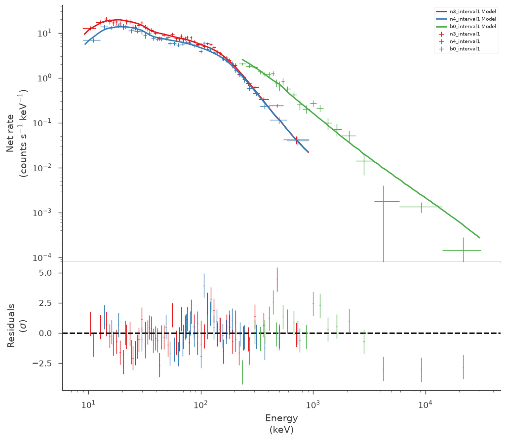
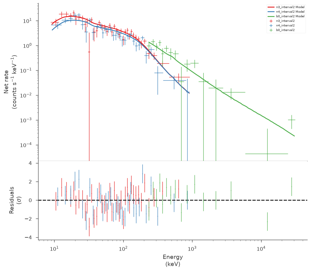
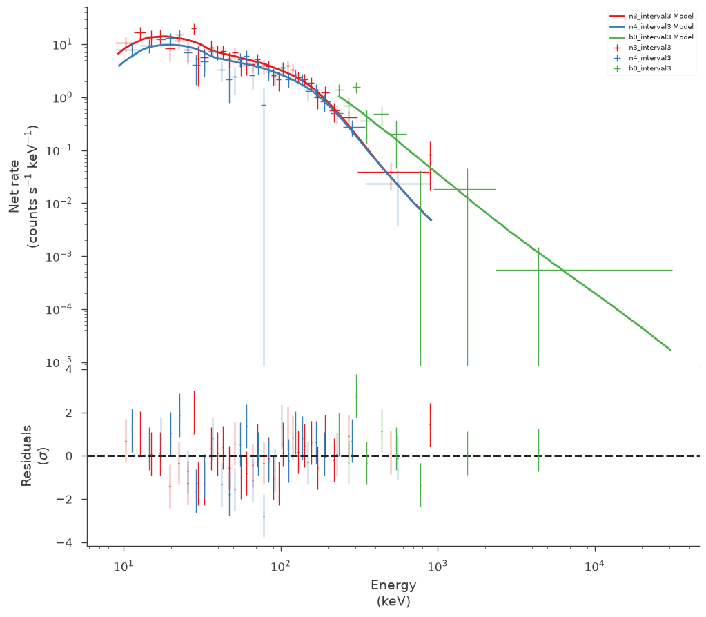
Examine the fits

Now we can look at the fits in count space to make sure they are ok.

[24]:

for a in analysis:
    a.restore_median_fit()
    _ = display_spectrum_model_counts(a, min_rate=[20, 20, 20], step=False)

         INFO      fit restored to median of posterior                                          sampler_base.py:157

         INFO      fit restored to median of posterior                                          sampler_base.py:157

         INFO      fit restored to median of posterior                                          sampler_base.py:157

17:53:16 INFO      fit restored to median of posterior                                          sampler_base.py:157

         INFO      fit restored to median of posterior                                          sampler_base.py:157

17:53:17 INFO      fit restored to median of posterior                                          sampler_base.py:157

         INFO      fit restored to median of posterior                                          sampler_base.py:157

         INFO      fit restored to median of posterior                                          sampler_base.py:157

17:53:18 INFO      fit restored to median of posterior                                          sampler_base.py:157

         INFO      fit restored to median of posterior                                          sampler_base.py:157

         INFO      fit restored to median of posterior                                          sampler_base.py:157

17:53:19 INFO      fit restored to median of posterior                                          sampler_base.py:157

../_images/notebooks_grb080916C_41_12.png

../_images/notebooks_grb080916C_41_13.png

../_images/notebooks_grb080916C_41_14.png

../_images/notebooks_grb080916C_41_15.png

../_images/notebooks_grb080916C_41_16.png

../_images/notebooks_grb080916C_41_17.png

../_images/notebooks_grb080916C_41_18.png

../_images/notebooks_grb080916C_41_19.png

../_images/notebooks_grb080916C_41_20.png

../_images/notebooks_grb080916C_41_21.png

../_images/notebooks_grb080916C_41_22.png

../_images/notebooks_grb080916C_41_23.png

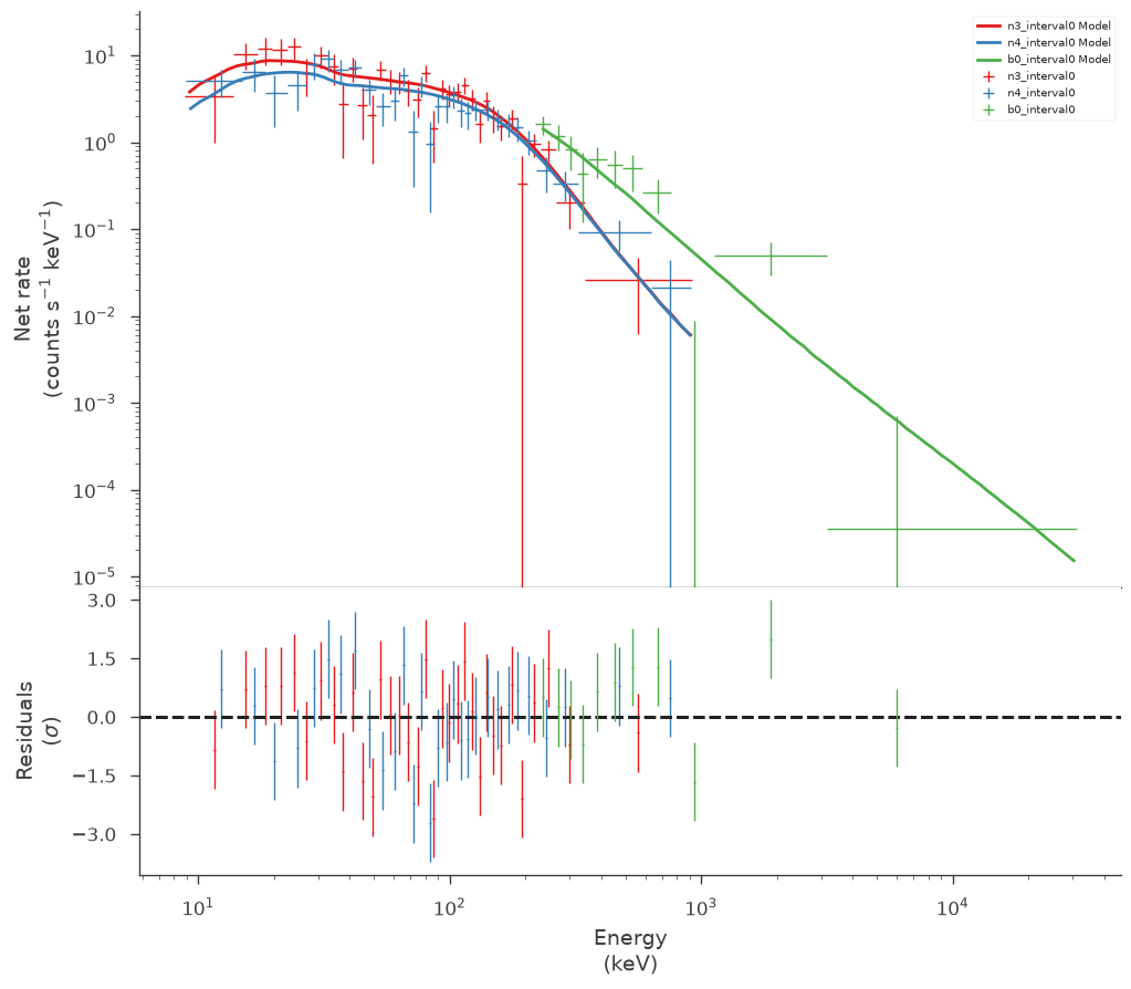
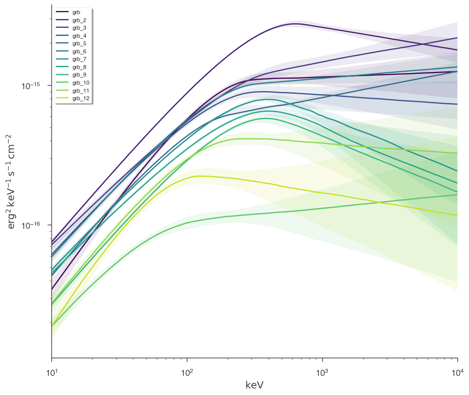
Finally, we can plot the models together to see how the spectra evolve with time.

[25]:

fig = plot_spectra(
    *[a.results for a in analysis[::1]],
    flux_unit="erg2/(cm2 s keV)",
    fit_cmap="viridis",
    contour_cmap="viridis",
    contour_style_kwargs=dict(alpha=0.1),
)

../_images/notebooks_grb080916C_43_13.png

This example can serve as a template for performing analysis on GBM data. However, as 3ML provides an abstract interface and modular building blocks, similar analysis pipelines can be built for any time series data.