Bayesian Sampler Examples

Examples of running each sampler avaiable in 3ML.

Before, that, let’s discuss setting up configuration default sampler with default parameters. We can set in our configuration a default algorithm and default setup parameters for the samplers. This can ease fitting when we are doing exploratory data analysis.

With any of the samplers, you can pass keywords to access their setups. Read each pacakges documentation for more details.

[1]:

from threeML import *
from threeML.plugins.XYLike import XYLike

from packaging.version import Version
import numpy as np
import dynesty
from jupyterthemes import jtplot

%matplotlib inline
jtplot.style(context="talk", fscale=1, ticks=True, grid=False)
silence_warnings()
set_threeML_style()

05:50:37 WARNING   The naima package is not available. Models that depend on it will not be         functions.py:43
                  available

         WARNING   The GSL library or the pygsl wrapper cannot be loaded. Models that depend on it  functions.py:65
                  will not be available.

         WARNING   The ebltable package is not available. Models that depend on it will not be     absorption.py:33
                  available

[2]:

threeML_config.bayesian.default_sampler

[2]:

<Sampler.emcee: 'emcee'>

[3]:

threeML_config.bayesian.emcee_setup

[3]:

{'n_burnin': None, 'n_iterations': 500, 'n_walkers': 50, 'seed': 5123}

If you simply run bayes_analysis.sample() the default sampler and its default parameters will be used.

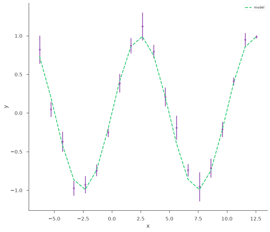
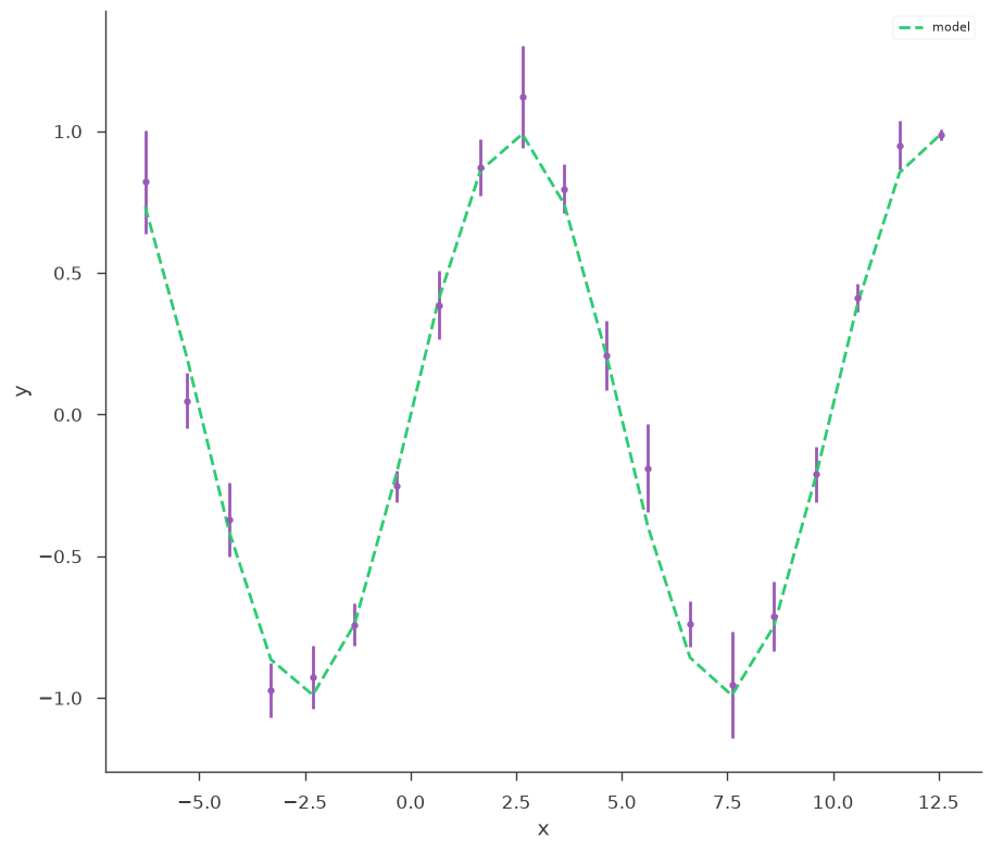
Let’s make some data to fit.

[4]:

sin = Sin(K=1, f=0.1)
sin.phi.fix = True
sin.K.prior = Log_uniform_prior(lower_bound=0.5, upper_bound=1.5)
sin.f.prior = Uniform_prior(lower_bound=0, upper_bound=0.5)

model = Model(PointSource("demo", 0, 0, spectral_shape=sin))

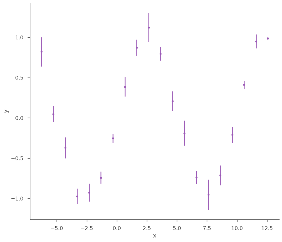
x = np.linspace(-2 * np.pi, 4 * np.pi, 20)
yerr = np.random.uniform(0.01, 0.2, 20)


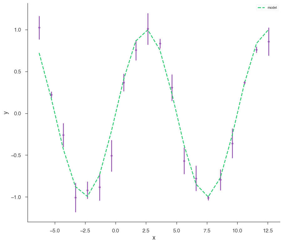
xyl = XYLike.from_function("demo", sin, x, yerr)
xyl.plot()

bayes_analysis = BayesianAnalysis(model, DataList(xyl))

05:50:39 INFO      Using Gaussian statistic (equivalent to chi^2) with the provided errors.            XYLike.py:90

05:50:40 INFO      Using Gaussian statistic (equivalent to chi^2) with the provided errors.            XYLike.py:90

../_images/notebooks_sampler_docs_5_2.png

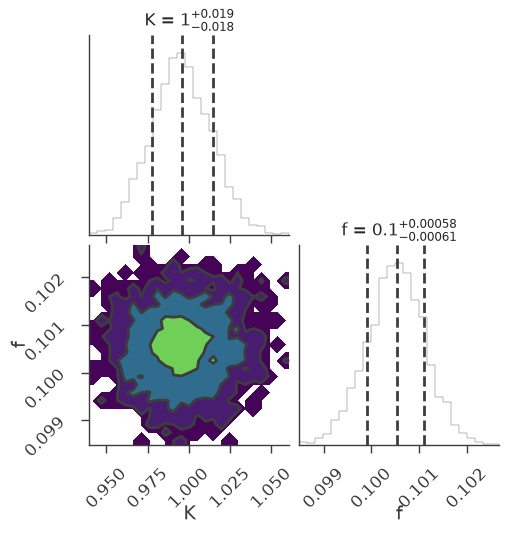
emcee

[5]:

bayes_analysis.set_sampler("emcee")
bayes_analysis.sampler.setup(n_walkers=20, n_iterations=500)
bayes_analysis.sample()

xyl.plot()
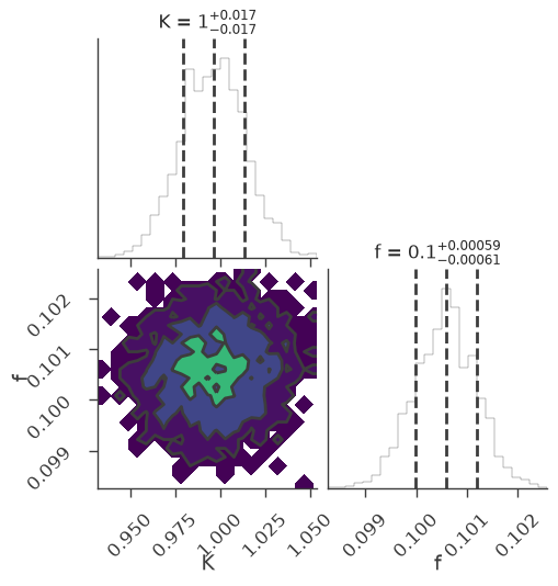
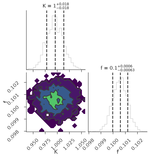
bayes_analysis.results.corner_plot()

         INFO      sampler set to emcee                                                    bayesian_analysis.py:186

05:50:41 INFO      Mean acceptance fraction: 0.7278                                            emcee_sampler.py:145

         INFO      fit restored to maximum of posterior                                         sampler_base.py:168

         INFO      fit restored to maximum of posterior                                         sampler_base.py:168

Maximum a posteriori probability (MAP) point:

	result	unit
parameter
demo.spectrum.main.Sin.K	1.033 +/- 0.026	1 / (keV s cm2)
demo.spectrum.main.Sin.f	(9.96 -0.08 +0.09) x 10^-2	rad / keV

Values of -log(posterior) at the minimum:

	-log(posterior)
demo	-9.038918
total	-9.038918

Values of statistical measures:

	statistical measures
AIC	22.783718
BIC	24.069300
DIC	21.971510
PDIC	1.942418

[5]:

../_images/notebooks_sampler_docs_7_12.png

../_images/notebooks_sampler_docs_7_13.png

../_images/notebooks_sampler_docs_7_14.png

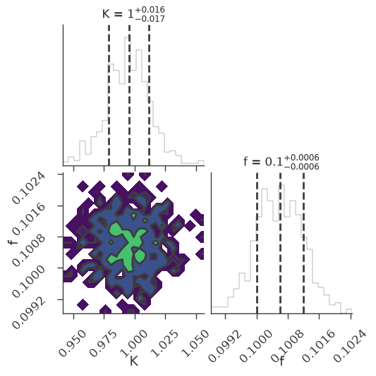
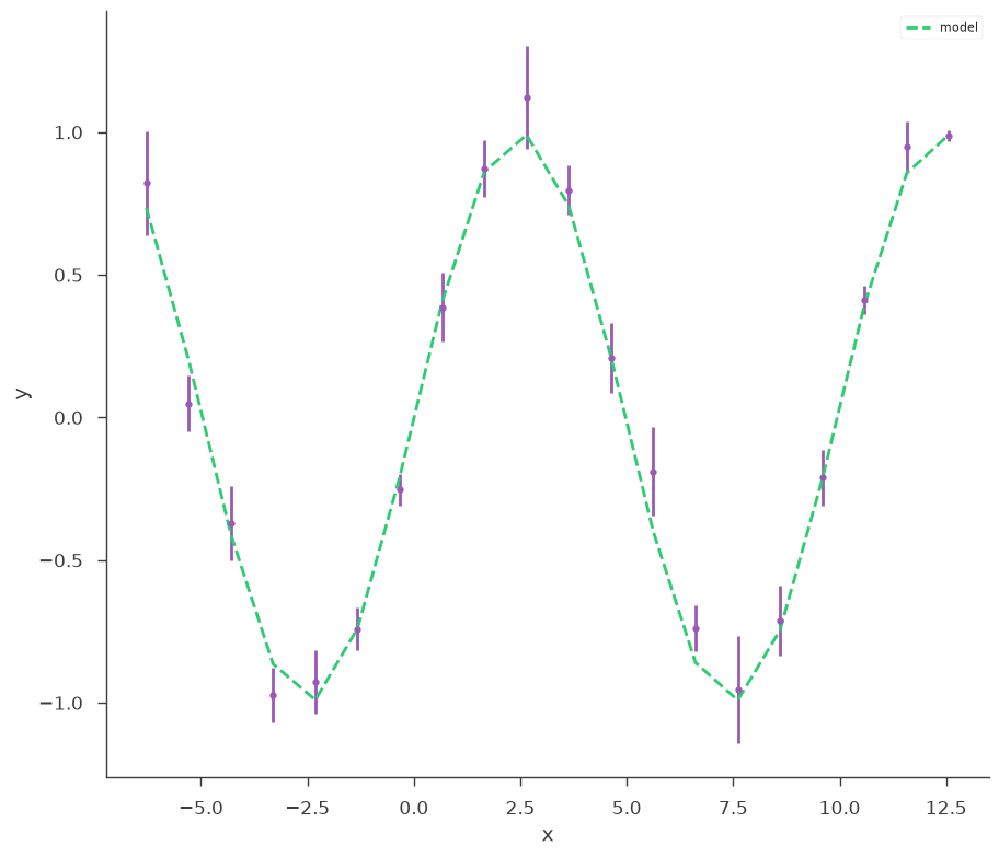
multinest

[6]:

bayes_analysis.set_sampler("multinest")
bayes_analysis.sampler.setup(n_live_points=400, resume=False, auto_clean=True)
bayes_analysis.sample()

xyl.plot()
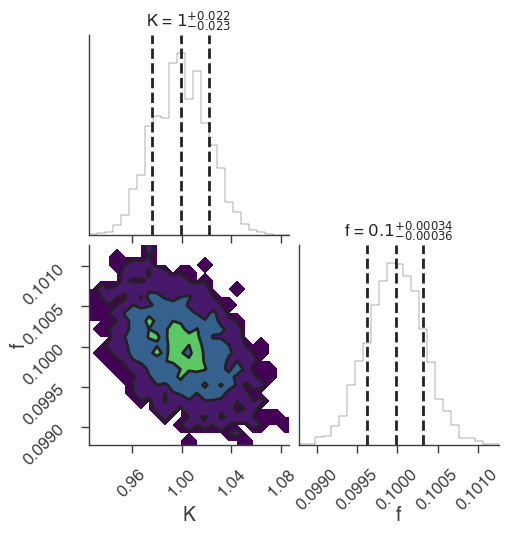
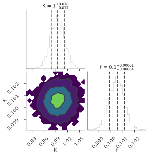
bayes_analysis.results.corner_plot()

05:50:42 INFO      sampler set to multinest                                                bayesian_analysis.py:186

 *****************************************************
 MultiNest v3.10
 Copyright Farhan Feroz & Mike Hobson
 Release Jul 2015

 no. of live points =  400
 dimensionality =    2
 *****************************************************

 MultiNest Warning!
 Parameter            1  of mode            3  is converging towards the edge of the prior.

 MultiNest Warning!
 Parameter            1  of mode            3  is converging towards the edge of the prior.
  analysing data from chains/fit-.txt ln(ev)=  -17.055684536516001      +/-  0.13268055531958889
 Total Likelihood Evaluations:         6008
 Sampling finished. Exiting MultiNest

05:50:43 INFO      fit restored to maximum of posterior                                         sampler_base.py:168

         INFO      fit restored to maximum of posterior                                         sampler_base.py:168

Maximum a posteriori probability (MAP) point:

	result	unit
parameter
demo.spectrum.main.Sin.K	1.032 -0.027 +0.028	1 / (keV s cm2)
demo.spectrum.main.Sin.f	(9.96 +/- 0.08) x 10^-2	rad / keV

Values of -log(posterior) at the minimum:

	-log(posterior)
demo	-9.039276
total	-9.039276

Values of statistical measures:

	statistical measures
AIC	22.784435
BIC	24.070017
DIC	22.119436
PDIC	2.020380
log(Z)	-7.407190

         INFO      deleting the chain directory chains                                     multinest_sampler.py:234

[6]:

../_images/notebooks_sampler_docs_9_11.png

../_images/notebooks_sampler_docs_9_12.png

../_images/notebooks_sampler_docs_9_13.png

dynesty

[7]:

bayes_analysis.set_sampler("dynesty_nested")
bayes_analysis.sampler.setup(nlive=400)
bayes_analysis.sample()

xyl.plot()
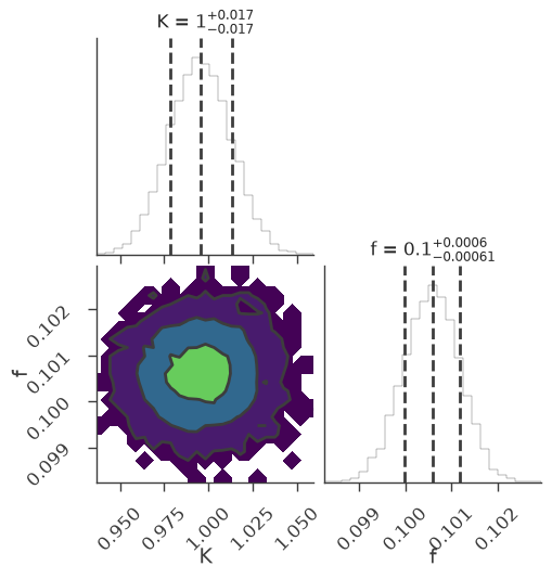
bayes_analysis.results.corner_plot()

         INFO      sampler set to dynesty_nested                                           bayesian_analysis.py:186

3765it [00:03, 1153.31it/s, +400 | bound: 10 | nc: 1 | ncall: 18053 | eff(%): 23.594 | loglstar:   -inf < -9.007 <    inf | logz: -17.371 +/-  0.136 | dlogz:  0.001 >  0.409]

05:50:46 INFO      fit restored to maximum of posterior                                         sampler_base.py:168

         INFO      fit restored to maximum of posterior                                         sampler_base.py:168

Maximum a posteriori probability (MAP) point:

	result	unit
parameter
demo.spectrum.main.Sin.K	1.033 -0.026 +0.027	1 / (keV s cm2)
demo.spectrum.main.Sin.f	(9.95 -0.09 +0.08) x 10^-2	rad / keV

Values of -log(posterior) at the minimum:

	-log(posterior)
demo	-9.039186
total	-9.039186

Values of statistical measures:

	statistical measures
AIC	22.784254
BIC	24.069836
DIC	22.086992
PDIC	2.004012
log(Z)	-7.544179

[7]:

../_images/notebooks_sampler_docs_11_10.png

../_images/notebooks_sampler_docs_11_11.png

../_images/notebooks_sampler_docs_11_12.png

[8]:

bayes_analysis.set_sampler("dynesty_dynamic")
bayes_analysis.sampler.setup()

if Version(dynesty.__version__) >= Version("3.0.0"):
    bayes_analysis.sample(n_effective=None)
else:
    bayes_analysis.sample(
        stop_function=dynesty.utils.old_stopping_function, n_effective=None
    )

xyl.plot()
bayes_analysis.results.corner_plot()

05:50:47 INFO      sampler set to dynesty_dynamic                                          bayesian_analysis.py:186

15823it [00:13, 1169.82it/s, batch: 8 | bound: 4 | nc: 1 | ncall: 37322 | eff(%): 42.334 | loglstar: -13.988 < -9.007 < -9.356 | logz: -17.398 +/-  0.070 | stop:  0.898]

05:51:01 INFO      fit restored to maximum of posterior                                         sampler_base.py:168

         INFO      fit restored to maximum of posterior                                         sampler_base.py:168

Maximum a posteriori probability (MAP) point:

	result	unit
parameter
demo.spectrum.main.Sin.K	1.033 +/- 0.027	1 / (keV s cm2)
demo.spectrum.main.Sin.f	(9.96 -0.09 +0.08) x 10^-2	rad / keV

Values of -log(posterior) at the minimum:

	-log(posterior)
demo	-9.038935
total	-9.038935

Values of statistical measures:

	statistical measures
AIC	22.783752
BIC	24.069334
DIC	22.071711
PDIC	1.996451
log(Z)	-7.543777

[8]:

../_images/notebooks_sampler_docs_12_10.png

../_images/notebooks_sampler_docs_12_11.png

../_images/notebooks_sampler_docs_12_12.png

zeus

[9]:

bayes_analysis.set_sampler("zeus")
bayes_analysis.sampler.setup(n_walkers=20, n_iterations=500)
bayes_analysis.sample()

xyl.plot()
bayes_analysis.results.corner_plot()

         INFO      sampler set to zeus                                                     bayesian_analysis.py:186

The run method has been deprecated and it will be removed. Please use the new run_mcmc method.
Initialising ensemble of 20 walkers...
Sampling progress : 100%|██████████| 625/625 [00:03<00:00, 170.26it/s]

05:51:05 INFO      fit restored to maximum of posterior                                         sampler_base.py:168

         INFO      fit restored to maximum of posterior                                         sampler_base.py:168

Summary
-------
Number of Generations: 625
Number of Parameters: 2
Number of Walkers: 20
Number of Tuning Generations: 38
Scale Factor: 1.249892
Mean Integrated Autocorrelation Time: 3.04
Effective Sample Size: 4112.68
Number of Log Probability Evaluations: 64917
Effective Samples per Log Probability Evaluation: 0.063353

None

Maximum a posteriori probability (MAP) point:

	result	unit
parameter
demo.spectrum.main.Sin.K	1.033 -0.027 +0.025	1 / (keV s cm2)
demo.spectrum.main.Sin.f	(9.96 -0.09 +0.08) x 10^-2	rad / keV

Values of -log(posterior) at the minimum:

	-log(posterior)
demo	-9.038916
total	-9.038916

Values of statistical measures:

	statistical measures
AIC	22.783714
BIC	24.069296
DIC	22.003078
PDIC	1.961844

[9]:

../_images/notebooks_sampler_docs_14_12.png

../_images/notebooks_sampler_docs_14_13.png

../_images/notebooks_sampler_docs_14_14.png

ultranest

[10]:

bayes_analysis.set_sampler("ultranest")
bayes_analysis.sampler.setup(
    min_num_live_points=400, frac_remain=0.5, use_mlfriends=False
)
bayes_analysis.sample()

xyl.plot()
bayes_analysis.results.corner_plot()

         INFO      sampler set to ultranest                                                bayesian_analysis.py:186

[ultranest] Sampling 400 live points from prior ...

[ultranest] Explored until L=-9
[ultranest] Likelihood function evaluations: 5391
[ultranest]   logZ = -17.19 +- 0.1132
[ultranest] Effective samples strategy satisfied (ESS = 974.8, need >400)
[ultranest] Posterior uncertainty strategy is satisfied (KL: 0.47+-0.09 nat, need <0.50 nat)
[ultranest] Evidency uncertainty strategy is satisfied (dlogz=0.42, need <0.5)
[ultranest]   logZ error budget: single: 0.13 bs:0.11 tail:0.41 total:0.42 required:<0.50
[ultranest] done iterating.

05:51:08 INFO      fit restored to maximum of posterior                                         sampler_base.py:168

         INFO      fit restored to maximum of posterior                                         sampler_base.py:168

Maximum a posteriori probability (MAP) point:

	result	unit
parameter
demo.spectrum.main.Sin.K	1.033 +/- 0.026	1 / (keV s cm2)
demo.spectrum.main.Sin.f	(9.95 -0.09 +0.08) x 10^-2	rad / keV

Values of -log(posterior) at the minimum:

	-log(posterior)
demo	-9.039284
total	-9.039284

Values of statistical measures:

	statistical measures
AIC	22.784450
BIC	24.070032
DIC	22.120489
PDIC	2.020420
log(Z)	-7.479574

[10]:

../_images/notebooks_sampler_docs_16_12.png

../_images/notebooks_sampler_docs_16_13.png

../_images/notebooks_sampler_docs_16_14.png