Example joint fit between GBM and Swift BAT

One of the key features of 3ML is the abil ity to fit multi-messenger data properly. A simple example of this is the joint fitting of two instruments whose data obey different likelihoods. Here, we have GBM data which obey a Poisson-Gaussian profile likelihoog ( PGSTAT in XSPEC lingo) and Swift BAT which data which are the result of a “fit” via a coded mask and hence obey a Gaussian ( \(\chi^2\) ) likelihood.

[1]:

import warnings

warnings.simplefilter("ignore")
import numpy as np

np.seterr(all="ignore")

[1]:

{'divide': 'warn', 'over': 'warn', 'under': 'ignore', 'invalid': 'warn'}

[2]:

%%capture
import matplotlib.pyplot as plt

np.random.seed(12345)
from threeML import *
from threeML.io.package_data import get_path_of_data_file
from threeML.io.logging import silence_console_log

[3]:

from jupyterthemes import jtplot

%matplotlib inline
jtplot.style(context="talk", fscale=1, ticks=True, grid=False)
set_threeML_style()
silence_warnings()

Plugin setup

We have data from the same time interval from Swift BAT and a GBM NAI and BGO detector. We have preprocessed GBM data to so that it is OGIP compliant. (Remember that we can handle the raw data with the TimeSeriesBuilder). Thus, we will use the OGIPLike plugin to read in each dataset, make energy selections and examine the raw count spectra.

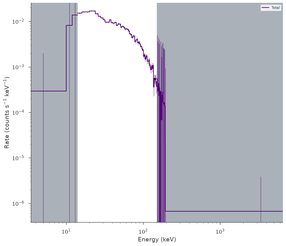
Swift BAT

[4]:

bat_pha = get_path_of_data_file("datasets/bat/gbm_bat_joint_BAT.pha")
bat_rsp = get_path_of_data_file("datasets/bat/gbm_bat_joint_BAT.rsp")

bat = OGIPLike("BAT", observation=bat_pha, response=bat_rsp)

bat.set_active_measurements("15-150")
bat.view_count_spectrum()

21:47:46 INFO      Auto-probed noise models:                                                    SpectrumLike.py:490

         INFO      - observation: gaussian                                                      SpectrumLike.py:491

         INFO      - background: None                                                           SpectrumLike.py:492

         INFO      Range 15-150 translates to channels 3-62                                    SpectrumLike.py:1247

[4]:

../_images/notebooks_joint_BAT_gbm_demo_7_4.png

../_images/notebooks_joint_BAT_gbm_demo_7_5.png

Fermi GBM

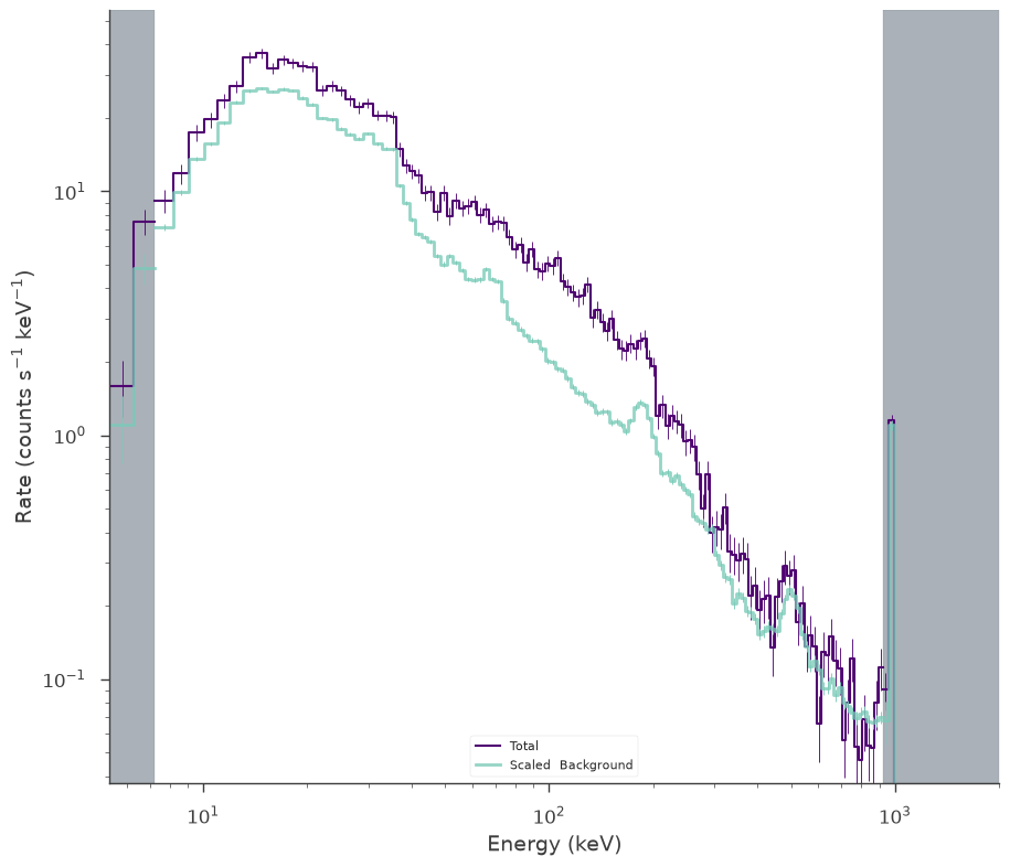
[5]:

nai6 = OGIPLike(
    "n6",
    get_path_of_data_file("datasets/gbm/gbm_bat_joint_NAI_06.pha"),
    get_path_of_data_file("datasets/gbm/gbm_bat_joint_NAI_06.bak"),
    get_path_of_data_file("datasets/gbm/gbm_bat_joint_NAI_06.rsp"),
    spectrum_number=1,
)


nai6.set_active_measurements("8-900")
nai6.view_count_spectrum()

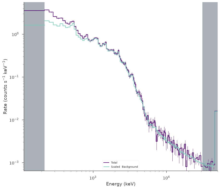
bgo0 = OGIPLike(
    "b0",
    get_path_of_data_file("datasets/gbm/gbm_bat_joint_BGO_00.pha"),
    get_path_of_data_file("datasets/gbm/gbm_bat_joint_BGO_00.bak"),
    get_path_of_data_file("datasets/gbm/gbm_bat_joint_BGO_00.rsp"),
    spectrum_number=1,
)

bgo0.set_active_measurements("250-30000")
bgo0.view_count_spectrum()

21:47:48 INFO      Auto-probed noise models:                                                    SpectrumLike.py:490

         INFO      - observation: poisson                                                       SpectrumLike.py:491

         INFO      - background: gaussian                                                       SpectrumLike.py:492

         INFO      Range 8-900 translates to channels 2-124                                    SpectrumLike.py:1247

         INFO      Auto-probed noise models:                                                    SpectrumLike.py:490

         INFO      - observation: poisson                                                       SpectrumLike.py:491

         INFO      - background: gaussian                                                       SpectrumLike.py:492

         INFO      Range 250-30000 translates to channels 1-119                                SpectrumLike.py:1247

[5]:

../_images/notebooks_joint_BAT_gbm_demo_9_8.png

../_images/notebooks_joint_BAT_gbm_demo_9_9.png

../_images/notebooks_joint_BAT_gbm_demo_9_10.png

Model setup

We setup up or spectrum and likelihood model and combine the data. 3ML will automatically assign the proper likelihood to each data set. At first, we will assume a perfect calibration between the different detectors and not a apply a so-called effective area correction.

[6]:

band = Band()

model_no_eac = Model(PointSource("joint_fit_no_eac", 0, 0, spectral_shape=band))

Spectral fitting

Now we simply fit the data by building the data list, creating the joint likelihood and running the fit.

No effective area correction

[7]:

data_list = DataList(bat, nai6, bgo0)

jl_no_eac = JointLikelihood(model_no_eac, data_list)

jl_no_eac.fit()

21:47:50 INFO      set the minimizer to minuit                                             joint_likelihood.py:1046

Best fit values:

	result	unit
parameter
joint_fit_no_eac.spectrum.main.Band.K	(2.75 +/- 0.06) x 10^-2	1 / (cm2 keV s)
joint_fit_no_eac.spectrum.main.Band.alpha	-1.029 +/- 0.017
joint_fit_no_eac.spectrum.main.Band.xp	(5.68 -0.35 +0.4) x 10^2	keV
joint_fit_no_eac.spectrum.main.Band.beta	-2.41 +/- 0.18

Correlation matrix:

1.00	0.90	-0.85	0.14
0.90	1.00	-0.73	0.08
-0.85	-0.73	1.00	-0.32
0.14	0.08	-0.32	1.00

Values of -log(likelihood) at the minimum:

	-log(likelihood)
BAT	53.059661
b0	553.066551
n6	761.164928
total	1367.291140

Values of statistical measures:

	statistical measures
AIC	2742.716960
BIC	2757.423988

[7]:

(                                                value  negative_error  \
 joint_fit_no_eac.spectrum.main.Band.K        0.027475       -0.000581
 joint_fit_no_eac.spectrum.main.Band.alpha   -1.029050       -0.017552
 joint_fit_no_eac.spectrum.main.Band.xp     567.524692      -34.825576
 joint_fit_no_eac.spectrum.main.Band.beta    -2.409243       -0.170842

                                            positive_error      error  \
 joint_fit_no_eac.spectrum.main.Band.K            0.000579   0.000580
 joint_fit_no_eac.spectrum.main.Band.alpha        0.017051   0.017301
 joint_fit_no_eac.spectrum.main.Band.xp          37.675189  36.250382
 joint_fit_no_eac.spectrum.main.Band.beta         0.185888   0.178365

                                                       unit
 joint_fit_no_eac.spectrum.main.Band.K      1 / (cm2 keV s)
 joint_fit_no_eac.spectrum.main.Band.alpha
 joint_fit_no_eac.spectrum.main.Band.xp                 keV
 joint_fit_no_eac.spectrum.main.Band.beta                    ,
        -log(likelihood)
 BAT           53.059661
 b0           553.066551
 n6           761.164928
 total       1367.291140)

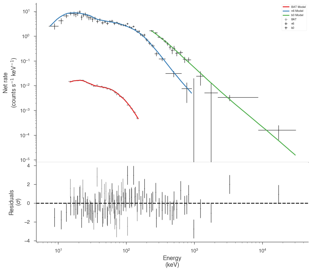
The fit has resulted in a very typical Band function fit. Let’s look in count space at how good of a fit we have obtained.

[8]:

threeML_config.plugins.ogip.fit_plot.model_cmap = "Set1"
threeML_config.plugins.ogip.fit_plot.n_colors = 3
display_spectrum_model_counts(
    jl_no_eac,
    min_rate=[0.01, 10.0, 10.0],
    data_colors=["grey", "k", "k"],
    show_background=False,
    source_only=True,
)

[8]:

../_images/notebooks_joint_BAT_gbm_demo_16_0.png

../_images/notebooks_joint_BAT_gbm_demo_16_1.png

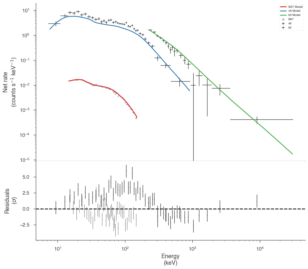
It seems that the effective areas between GBM and BAT do not agree! We can look at the goodness of fit for the various data sets.

[9]:

gof_object = GoodnessOfFit(jl_no_eac)

gof, res_frame, lh_frame = gof_object.by_mc(n_iterations=100)

[10]:

import pandas as pd

pd.Series(gof)

[10]:

total    0.00
BAT      0.00
n6       0.00
b0       0.56
dtype: float64

Both the GBM NaI detector and Swift BAT exhibit poor GOF.

With effective are correction

Now let’s add an effective area correction between the detectors to see if this fixes the problem. The effective area is a nuissance parameter that attempts to model systematic problems in a instruments calibration. It simply scales the counts of an instrument by a multiplicative factor. It cannot handle more complicated energy dependent

[11]:

# turn on the effective area correction and set it's bounds
nai6.use_effective_area_correction(0.2, 1.8)
bgo0.use_effective_area_correction(0.2, 1.8)

model_eac = Model(PointSource("joint_fit_eac", 0, 0, spectral_shape=band))

jl_eac = JointLikelihood(model_eac, data_list)

jl_eac.fit()

21:48:21 INFO      n6 is using effective area correction (between 0.2 and 1.8)                 SpectrumLike.py:2279

         INFO      b0 is using effective area correction (between 0.2 and 1.8)                 SpectrumLike.py:2279

         INFO      set the minimizer to minuit                                             joint_likelihood.py:1046

Best fit values:

	result	unit
parameter
joint_fit_eac.spectrum.main.Band.K	(2.98 -0.11 +0.12) x 10^-2	1 / (cm2 keV s)
joint_fit_eac.spectrum.main.Band.alpha	(-9.84 +/- 0.26) x 10^-1
joint_fit_eac.spectrum.main.Band.xp	(3.31 -0.30 +0.33) x 10^2	keV
joint_fit_eac.spectrum.main.Band.beta	-2.36 +/- 0.15
cons_n6	1.56 +/- 0.04
cons_b0	1.41 +/- 0.10

Correlation matrix:

1.00	0.95	-0.92	0.31	0.29	0.62
0.95	1.00	-0.83	0.26	0.26	0.52
-0.92	-0.83	1.00	-0.36	-0.45	-0.77
0.31	0.26	-0.36	1.00	0.04	-0.03
0.29	0.26	-0.45	0.04	1.00	0.47
0.62	0.52	-0.77	-0.03	0.47	1.00

Values of -log(likelihood) at the minimum:

	-log(likelihood)
BAT	40.069813
b0	544.753755
n6	644.708495
total	1229.532064

Values of statistical measures:

	statistical measures
AIC	2471.348873
BIC	2493.326689

[11]:

(                                             value  negative_error  \
 joint_fit_eac.spectrum.main.Band.K        0.029804       -0.001155
 joint_fit_eac.spectrum.main.Band.alpha   -0.984159       -0.025655
 joint_fit_eac.spectrum.main.Band.xp     331.187717      -29.353362
 joint_fit_eac.spectrum.main.Band.beta    -2.359197       -0.153746
 cons_n6                                   1.562228       -0.037619
 cons_b0                                   1.408389       -0.095096

                                         positive_error      error  \
 joint_fit_eac.spectrum.main.Band.K            0.001197   0.001176
 joint_fit_eac.spectrum.main.Band.alpha        0.026221   0.025938
 joint_fit_eac.spectrum.main.Band.xp          32.991780  31.172571
 joint_fit_eac.spectrum.main.Band.beta         0.152670   0.153208
 cons_n6                                       0.038849   0.038234
 cons_b0                                       0.095033   0.095065

                                                    unit
 joint_fit_eac.spectrum.main.Band.K      1 / (cm2 keV s)
 joint_fit_eac.spectrum.main.Band.alpha
 joint_fit_eac.spectrum.main.Band.xp                 keV
 joint_fit_eac.spectrum.main.Band.beta
 cons_n6
 cons_b0                                                  ,
        -log(likelihood)
 BAT           40.069813
 b0           544.753755
 n6           644.708495
 total       1229.532064)

Now we have a much better fit to all data sets

[12]:

display_spectrum_model_counts(
    jl_eac, step=False, min_rate=[0.01, 10.0, 10.0], data_colors=["grey", "k", "k"]
)

[12]:

../_images/notebooks_joint_BAT_gbm_demo_24_0.png

../_images/notebooks_joint_BAT_gbm_demo_24_1.png

[13]:

gof_object = GoodnessOfFit(jl_eac)

# for display purposes we are keeping the output clear
# with silence_console_log(and_progress_bars=False):
gof, res_frame, lh_frame = gof_object.by_mc(n_iterations=100, continue_on_failure=True)

[14]:

import pandas as pd

pd.Series(gof)

[14]:

total    0.89
BAT      0.35
n6       0.89
b0       0.87
dtype: float64

Examining the differences

Let’s plot the fits in model space and see how different the resulting models are.

[15]:

plot_spectra(
    jl_eac.results,
    jl_no_eac.results,
    fit_cmap="Set1",
    contour_cmap="Set1",
    flux_unit="erg2/(keV s cm2)",
    equal_tailed=True,
)

[15]:

../_images/notebooks_joint_BAT_gbm_demo_28_3.png

../_images/notebooks_joint_BAT_gbm_demo_28_4.png

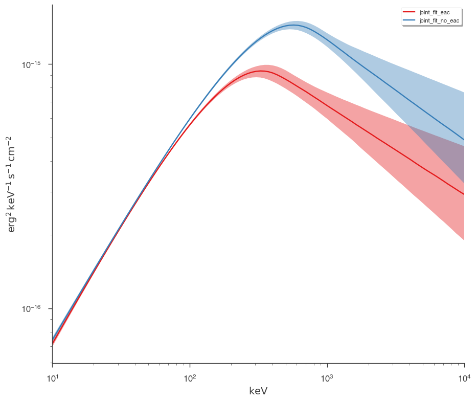
We can easily see that the models are different